In this bio-recipe we construct a class for discrete Bayesian networks. Bayesian networks are really a subset of the category of graphical models. Graphical models combine probability theory and graph theory. These models are useful because they provide an intuitive graphical representation of a joint probability distribution over a large number of random variables. Any joint probability distribution can be visualized by a graph G = (V, E) consisting of a set of vertices (V) and a set of Edges (E). The vertices or nodes in the graph symbolize the random variables. Two nodes in the graph are joined by an edge whenever the two random variables depend on each other in a stochastic sense. Consequently, the lack of an edge between two nodes represents conditional independence between the two nodes.
A more comprehensive description of Bayesian networks and graphical models is given by Kevin Murphy.
As already mentioned Bayesian networks (also known as Belief Networks) are a subset of the larger class of graphical models, namely the subset that uses directed acyclic graphs (DAG) to represent joint probability distributions. That means the independence assumptions take the directionality of arcs into account. To define a Bayesian network, one has to specify the structure and the parameters.
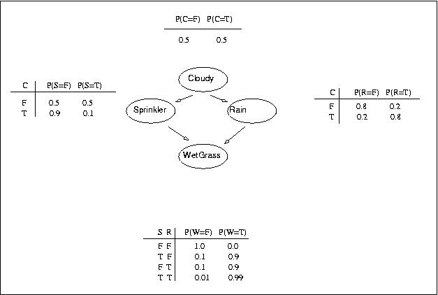
To illustrate the main concepts we consider the same example as Kevin Murphy did in his description. The following figure shows the graph structure and the assumed input parameters.
The example used here is well known under the name 'Sprinkler example'. The network consists of 4 nodes and it models possible causes of grass being wet (WetGrass). The grass can either be wet because of rain (Rain) or because the sprinkler was on (Sprinkler). Clouds in the sky (Cloudy) influence both Sprinker and Rain.
We assign the total number of nodes to the variable N and encode the nodes with integers from 1 to 4. The nodes must always be sorted in topological order, i.e., ancestor nodes must precede the descendants.
N := 4:
C := 1:
S := 2:
R := 3:
W := 4:
The topology of our network is defined by a directed acyclic graph (DAG). We use an adjacency matrix to specify the DAG in our example. An adjacency matrix has dimension N-by-N and any given element in row i and column j is 1, if node i is connected to node j by a directed arc. Elements that correspond to node pairs without a directed arc between them are 0. Four our example, we can construct the adjacency matrix as follows:
dag := CreateArray(1..N,1..N):
dag[C,R] := 1:
dag[C,S] := 1:
dag[R,W] := 1:
dag[S,W] := 1:
print(dag):
 0 1 1 0
 0 0 0 1
 0 0 0 1
 0 0 0 0
In addition to specifying the graph structure, we must also specify the size of each node. The size of a node is defined as the number of possible states it can take. In our example, we assume all nodes to be binary. At this point we also make the rather random assignment of 'false' corresponding to 1 and 'true' corresponding to 2.
node_sizes:=2*[seq(1,N)]:
Now we are ready to construct our Bayesian network class which we call BayesNet. The constructor of the BayesNet class looks as follows:
BayesNet:= proc( AdjMat:matrix(numeric), NodeSize:list(posint), NodeName:list(string),
                 ObsNode:list(posint), parents:list, CPD:list ) option polymorphic;
where AdjMat contains the adjacency matrix, NodeSize the vector with the sizes of the nodes, NodeName the vector of the names of the node, ObsNode the vector with indices of the observed nodes, parents a list of which each element consists of all parents for the respective node, and CPD the conditional probability distributions.
  # check for correct number of arguments
  if nargs < 2 or nargs > 4 then
    error('Wrong number of arguments for BayesNet:',
          'Number of arguments specified: ', nargs,
          'Usage: BayesNet( AdjMat, NodeSize )'):
  else
    # assign number of nodes to n, initialize field CPD
    #  to an array of size n
    n := length(AdjMat):
    icpd := CreateArray( 1..n, [] ):
    # parse arguments
    if nargs = 2 then
      noeval( BayesNet( AdjMat, NodeSize, '', [], [], icpd ) ):
    elif nargs = 3 then
      noeval( BayesNet( AdjMat, NodeSize, NodeName, [], [], icpd ) ):
    elif nargs = 4 then
      noeval( BayesNet( AdjMat, NodeSize, NodeName, ObsNode, [], icpd ) ):
    fi:
  fi:
end:
After having defined the BayesNet class, we can create an instance of this class by just calling the class name with the appropriate arguments.
BNet := BayesNet( dag, node_sizes );
BNet := BayesNet([[0, 1, 1, 0], [0, 0, 0, 1], [0, 0, 0, 1], [0, 0, 0, 0]],[2, 2,
2, 2],,[],[],[[], [], [], []])
The type checking within the BayesNet constructor and the last elif-statement ensure that we can only call BayesNet with a number of arguments between 2 and 4. This means that we do not allow the specification of the conditional probability distributions within the constructor. Their specification will be done in a separate method. If BayesNet is called with less than 2 or more than 4 arguments, it will produce an error message similar to the following:
BNet0 := BayesNet();
Error, (in BayesNet) Wrong number of arguments for BayesNet:,
Number of arguments specified: , 0, Usage: BayesNet( AdjMat, NodeSize )
It is possible and also advisable to associate names with the nodes. If omitted the names are by default just an empty field. Node names are best specified as a vector of strings. For our example this could look like:
node_names := ['Cloudy','Sprinkler','Rain','WetGrass']:
The above specified node names can then be used as an argument to BayesNet.
BNet := BayesNet( dag, node_sizes, node_names );
BNet := BayesNet([[0, 1, 1, 0], [0, 0, 0, 1], [0, 0, 0, 1], [0, 0, 0, 0]],[2, 2,
2, 2],[Cloudy, Sprinkler, Rain, WetGrass],[],[],[[], [], [], []])
For all the nodes in the network that we have observed data, we have to indicate their index in a vector and pass it as the fourth argument to BayesNet constructor. As an example, let us assume that we have observed data for the 'Cloudy' and the 'WetGrass' nodes, then we would specify this as follows:
obs_nodes := [1, 4]:
BNet := BayesNet( dag, node_sizes, node_names, obs_nodes );
BNet := BayesNet([[0, 1, 1, 0], [0, 0, 0, 1], [0, 0, 0, 1], [0, 0, 0, 0]],[2, 2,
2, 2],[Cloudy, Sprinkler, Rain, WetGrass],[1, 4],[],[[], [], [], []])
The class definition of BayesNet allows us to use AdjMat, NodeSize, NodeName, ObsNode, parents, and CPD as selectors without any need of defining a specific selector method called BayesNet_select. Using each of the selectors specified in the constructor returns the respective content of the selected field, and looks as follows:
print(BNet[AdjMat]);
 0 1 1 0
 0 0 0 1
 0 0 0 1
 0 0 0 0
BNet[NodeName];
[Cloudy, Sprinkler, Rain, WetGrass]
BNet[ObsNode];
[1, 4]
BNet[parents];
[]
BNet[CPD];
[[], [], [], []]
When working with Bayesian networks, we often need to know the parent nodes of a given node. Hence, it is convenient to have a method that operates on the BayesNet object and returns for each node a list with the parent nodes.
GetParents := proc( BN )
  # extract adjacency matrix and the number of nodes
  am := BN[AdjMat]:
  n := length(am):
  # initialize an array to store the parents
  p := CreateArray( 1..n ):
  # loop over all nodes and search for entries in
  # the adjacency matrix = 1. This loop is done
  # column-wise, because the adjacency matrix is
  # upper-triangular
  for i to n do
    # extract column vector i out of am
    cvi := [seq(am[irow,i],irow=1..n)]:
    # search in cvi for all entries = 1
    p[i] := SearchAllArray( 1, cvi ):
  od:
  return(p):
end:
The result of the method GetParents is stored in the parents field of the BayesNet object.
BNet[parents] := GetParents(BNet);
BNet[parents] := [[], [1], [1], [2, 3]]
The parameters of a graphical model are represented by the conditional probabilities (CPD) of each node given its parents. The simplest form of CPD is a table, which is suitable when all the nodes are discrete-valued. Tabular CPDs, also called conditional probability tables (CPT), are stored as multidimensional arrays. Note that the CPT have to be specified such that the index of the node toggles fastest and the index of the first parents toggles slowest.
ConProDistr := CreateArray( 1..N ):
ConProDistr[C] := [0.5, 0.5]:
ConProDistr[S] := [0.5, 0.5, 0.9, 0.1]:
ConProDistr[R] := [0.8, 0.2, 0.2 ,0.8]:
ConProDistr[W] := [1, 0, 0.1, 0.9, 0.1, 0.9, 0.01, 0.99]:
The array 'ConProDistr' contains on each row the conditional probabilities of each node given its parent nodes. For nodes that do not have any parents the row in 'ConProDistr' contains just the prior probabilities. The CPTs that we have specified above, can easily be visualized by converting them into Darwin tables. In order to prepare this conversion, we first write two procedures that will be needed for the conversion. The first procedure computes for a given node the total number of possible state combinations for the node and all its parent nodes. The second procedure generates one state combination for a node and its parent nodes at the time.
GetTotalNrStateComb := proc( BN, node:integer )
  # extract the parents of node from BN
  pn := BN[parents,node]:
  # if node has no parents, just return its node size
  if pn = [] then
    return(BN[NodeSize,node]):
  else
    # compute product of node sizes of parents and node
    tnsc := 1:
    for i to length(pn) do
      tnsc := tnsc * BN[NodeSize,pn[i]]:
    od:
    tnsc := tnsc * BN[NodeSize,node]:
    return(tnsc):
  fi:
end:
The above procedure extracts the parents of the node we are interested in. If this node has no parents the total number of state combinations is just its node size. Otherwise the product over the node sizes of the parent nodes and its own node size is computed and returned. So far we have just computed how many possible state combinations we can have looking at a given node and its parents. This number determines the number of rows that the Darwin table to represent the CPT for a given node has. Now we have to generate all possible combinations.
CreateStatComb := proc( cidx:integer, vstate:array(numeric) )
  # determine length of array to be returned = length of vstate
  lsc := length(vstate):
  # if only two arguments are specified, then we are at the beginning
  if nargs = 2 then
    # initialize array for states to be returned, and position within
    #  vstcomb to the last position
    vstcomb := CreateArray( 1..lsc ):
    pos := lsc:
  else
    # more than two arguments were specified, so this proc has been
    #  called before, the position w/in vstcomb is the 3rd argument
    pos := args[3]:
    # all other args are the states that are already determined
    #  w/in vstcomb
    vstcomb := args[4]:
  fi:
  # compute state value at current position
  vstcomb[pos] := mod(cidx,vstate[pos]):
  # if the index cidx is smaller than the node size in vstate[pos],
  #  then there is not point to continue here, just return what we
  #  have.
  if cidx < vstate[pos] then
    return(vstcomb):
  fi:
  # check whether we are already at the beginning of vstcomb
  #  we are building vstcomb in reverse, i.e. from last element
  #  to the first
  if pos > 1 then
    # if the integer quotient is less then the node size at pos-1
    #  then we are done
    if iquo(cidx,vstate[pos]) < vstate[pos-1] then
      vstcomb[pos-1] := iquo(cidx,vstate[pos]):
      return(vstcomb):
    else
      # iquo is larger than node size at pos-1, recurse
      CreateStatComb( iquo(cidx,vstate[pos]), vstate, (pos-1), vstcomb ):
    fi:
  else
    return(vstcomb):
  fi:
end:
The procedure 'CreateStatComb' aims at generating a certain combination of states of a given node and its parent nodes. When called in a loop over all integers between 1 and the total number of state combinations, the result will be all possible state combinations of the node and its parents. Please note that the ordering of parents has to be consistent with the ordering in the BayesNet class. The node has to be specified last. The generated states will now be used in the conversion procedure which follows next.
ConvertCPT := proc( BN, Node, CPT )
  # get the parents of Node
  pn := BN[parents,Node]:
  # convert CPT into tables
  # determine how many columns we need,
  #  each parent, the node, and the entry of the CPT
  #  need a column
  nc := length(pn) + 2:
  # depending on whether the current node has parents
  #  or not, the first row looks different
  frow := Row():
  if pn = [] then
    frow := Row(BN[NodeName,Node], 'CPD('.BN[NodeName,Node].')'):
  else
    for j to length(pn) do
      frow := append(frow, BN[NodeName,pn[j]]):
    od:
    frow := append(frow, BN[NodeName,Node], 'CPD('.BN[NodeName,Node].')'):
  fi:
  # set up the table entry for Node title and first row
  CPTable := Table(center, border, ColAlign(seq('c',nc)),
                   title=sprintf('Conditional Probability Table for Node: %s',
                                 BN[NodeName,Node]), frow):
  # the number of rows that follow now, depends on
  #  the number of parents and the node sizes. It is computed
  #  using the procedure GetTotalNrStateComb.
  nrow := GetTotalNrStateComb( BNet, Node ):
  # determine vector of node sizes for current node and its parents
  nscn := CreateArray( 1..(length(pn)+1) ):
  nscn[length(nscn)] := BN[NodeSize,Node]:
  # determine node size for parents only, if i has parents
  if pn <> [] then
    for k to length(pn) do
      nscn[k] := BN[NodeSize,pn[k]]:
    od:
  fi:
  # now we loop over all combinations and add a row
  for l to nrow do
    CPTable := append(CPTable, Row(op(CreateStatComb(l-1, nscn) + [seq(1,length(nscn))]), CPT[l])):
  od:
  return(CPTable):
end:
The result of the conversion can now be shown by first calling the conversion procedure, and then performing a loop over all nodes and printing the tables.
for node in [C, S, R, W] do
  print( ConvertCPT( BNet, node, ConProDistr[node] ) ):
od:
  Conditional Probability Table for Node: Cloudy


                           -------------------------
                           |  Cloudy  CPD(Cloudy)  |
                           |    1         0.5      |
                           |    2         0.5      |
                           -------------------------

  Conditional Probability Table for Node: Sprinkler


                    ---------------------------------------
                    |  Cloudy  Sprinkler  CPD(Sprinkler)  |
                    |    1         1           0.5        |
                    |    1         2           0.5        |
                    |    2         1           0.9        |
                    |    2         2           0.1        |
                    ---------------------------------------

  Conditional Probability Table for Node: Rain


                         -----------------------------
                         |  Cloudy  Rain  CPD(Rain)  |
                         |    1      1       0.8     |
                         |    1      2       0.2     |
                         |    2      1       0.2     |
                         |    2      2       0.8     |
                         -----------------------------

  Conditional Probability Table for Node: WetGrass


                 ----------------------------------------------
                 |  Sprinkler  Rain  WetGrass  CPD(WetGrass)  |
                 |      1       1       1            1        |
                 |      1       1       2            0        |
                 |      1       2       1           0.1       |
                 |      1       2       2           0.9       |
                 |      2       1       1           0.1       |
                 |      2       1       2           0.9       |
                 |      2       2       1          0.01       |
                 |      2       2       2          0.99       |
                 ----------------------------------------------
So far, we have specified the parameters (CPD). Now we have to enter them into the BayesNet object. In the class declaration of BayesNet, we have reserved a field called 'CPD' which is now used to store the parameters belonging to the Bayesian network. The parameters are entered into the BayesNet using the procedure 'EnterCPD'. This procedure enters the parameters for just one node at the time. To enter all parameters of the network, the procedure has to be called for all nodes subsequently. This allows us to update parameters later using this same procedure.
EnterTabularCPD := proc( BN, Node, CPT )
  # get the node size of Node, and verify whether entries in CPT
  #  are consistent, i.e. probabilities sum up to 1 and the order
  #  in which they are specified is correct, if not throw an error.
  nsn := BN[NodeSize,Node]:
  # groups of elements of nsn in CPT have to sum up to 1.
  for k to iquo(length(CPT), nsn) do
    if sum(CPT[(k-1)*nsn+1..k*nsn]) <> 1 then
      error('CPD not consistent at state: ', k, ' of node: ', Node):
    fi:
  od:
  # get the parents of Node
  pn := BN[parents, Node]:
  # for all nodes without parents, CPT is returned as
  #  the parameter.
  if pn = [] then
    return(CPT):
  else
    # for all nodes with parents, CPT has to be reshaped
    #  according to the node sizes of parents and Node
    # determine vector of node sizes
    nscn := CreateArray( 1..(length(pn)+1) ):
    nscn[length(nscn)] := nsn:
    for k to length(pn) do
      nscn[k] := BN[NodeSize,pn[k]]:
    od:
    return(ReshapeArray(CPT, nscn)):
  fi:
end:
We can now enter the specified parameters into our BayesNet object using the following command:
for node in [C, S, R, W] do
  BNet[CPD,node] := EnterTabularCPD( BNet, node, ConProDistr[node] );
od;
BNet[CPD,1] := [0.5000, 0.5000]
BNet[CPD,2] := [[0.5000, 0.5000], [0.9000, 0.10000000]]
BNet[CPD,3] := [[0.8000, 0.2000], [0.2000, 0.8000]]
BNet[CPD,4] := [[[1, 0], [0.10000000, 0.9000]], [[0.10000000, 0.9000], [
0.01000000, 0.9900]]]
Now we are done with creating a BayesNet object. We have specified the structure of the network and entered the parameters of the network. If we want to check all our entries, we can just enter the name of our BayesNet object at the Darwin prompt.
BNet;
BayesNet([[0, 1, 1, 0], [0, 0, 0, 1], [0, 0, 0, 1], [0, 0, 0, 0]],[2, 2, 2, 2],[
Cloudy, Sprinkler, Rain, WetGrass],[1, 4],[[], [1], [1], [2, 3]],[[0.5000,
0.5000], [[0.5000, 0.5000], [0.9000, 0.10000000]], [[0.8000, 0.2000], [0.2000,
0.8000]], [[[1, 0], [0.10000000, 0.9000]], [[0.10000000, 0.9000], [0.01000000,
0.9900]]]])
In order to produce a nicely structured view of the BayesNet object we define a print method.
BayesNet_print := proc( BN ) option internal;
  printf('\n\n'):
  printf('                 Node Names:  %a\n', BN[NodeName]):
  printf('           Adjacency Matrix:  %a\n', BN[AdjMat]):
  printf('                 Node Sizes:  %a\n', BN[NodeSize]):
  printf('             Observed Nodes:  %a\n', BN[ObsNode]):
  printf('                    Parents:  %a\n', BN[parents]):
  printf('  Conditional Probabilities:  [1 x %d multi-dim array]\n', length(BN[CPD])):
  printf('\n'):
end:
Calling the print with the BayesNet object as an argument produces a nice output.
print( BNet ):
                 Node Names:  [Cloudy, Sprinkler, Rain, WetGrass]
           Adjacency Matrix:  [[0, 1, 1, 0], [0, 0, 0, 1], [0, 0, 0, 1], [0, 0, 0, 0]]
                 Node Sizes:  [2, 2, 2, 2]
             Observed Nodes:  [1, 4]
                    Parents:  [[], [1], [1], [2, 3]]
  Conditional Probabilities:  [1 x 4 multi-dim array]
© 2005 by Laura Bosia and Peter von Rohr, Informatik, ETH Zurich
Authors: Laura Bosia & Peter von Rohr
Last updated on Fri Sep 2 16:59:00 2005 by PvR