Traditionally, proteins were identified by de novo sequencing, notably via the Edman degradation. As the protein databases grew, correlating experimental information with the information in sequence databases provided a faster means of identification. Mass spectrometry provides a set of weights of protein fragments which can be compared to existing sequence databases. This procedure, called mass mapping, is a very effective means of identifying proteins. This method described here is not effective to find the composition of an unknown protein (a separate field of study), but it is effective in locating an unknown sample if its sequence is recorded in a protein database. For a review of the use of mass spectrometry in proteomics, see Chem. Rev. 2001, 101, 269-295 by Aebersold and Goodlett.
One of the ways of breaking a protein into smaller pieces according to a certain pattern is by using enzymes which digest the protein. For example, trypsin breaks a protein after every Arginine (R) or after every Lysine (K) not followed by a Proline (P). It is not very difficult, given the rules, to write a function which will do the theoretical digestion of a sequence. The function for trypsin is:
DigestTrypsin := proc( s:string )
description 'break a peptide sequence as if digested by trypsin';
res := NULL;
i := 1;
# the fragments will be defined between i and j
for j to length(s)-1 do
    if s[j] = 'R' or s[j] = 'K' and s[j+1] <> 'P' then
        res := res, s[i..j];
        i := j+1
        fi
    od;
# collect the last fragment
[res, s[i..-1]]
end:
If we would subject the protein
p := 'YKVTLVDQRREGDIAEDQGLDLKPYSCRAGACSTCAGKIVSGDLDDDQIEKG':
to the action of trypsin, we obtain 7 fragments:
dp := DigestTrypsin(p);
dp := [YK, VTLVDQR, R, EGDIAEDQGLDLKPYSCR, AGACSTCAGK, IVSGDLDDDQIEK, G]
The molecular weight of fragments can be found experimentally by mass spectrometry methods to a good level of accuracy. More importantly, mass spectrometry requires very small samples in the order of fractions of picomoles. In Darwin we can compute the theoretical molecular mass of a protein sequence by using the function GetMolWeight
GetMolWeight(dp);
[309.3440, 829.8990, 174.1880, 2009.1640, 867.9860, 1446.5000, 75.0520]
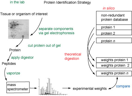
The problem of identifying a sampled protein can be reduced to digesting the protein with an enzyme, finding the molecular weights of each of the pieces (in the lab), digesting in silico each of the proteins in a database to generate for each protein a list of theoretical masses, and then comparing the experimentally measured weights with the theoretical weights of the proteins in the database. The process can be repeated with several different enzymes to increase its selectivity.
The purpose of this biorecipe is to describe an algorithm to perform this matching against the database in an efficient way. Secondly we are interested in estimating when a match of weights is significant. This algorithm is available in Darwin under the name SearchMassDb. Readers interested just in its use should skip to the example section. The next sections describe the algorithm and its theoretical basis.
If our mass measures were perfect and our sequence database contained all searched sequences, this would be an almost trivial problem. Search a vector of weights against all possible vectors of weights computed from the sequence database. This problem is known in computer science as multidimensional search. This is, unfortunately, not the case for the following reasons:
| (a) | The recording of molecular mass is subject to a relative error, in general less than 1% but not exact enough as to identify even very short sequences of amino acids. |
| (b) | Two of the amino acids, leucine and isoleucine, are composed of the same atoms and thus have identical weights. In addition, Lysine (molecular weight, 146.1740) and Glutamine (molecular weight, 146.1310) have very close molecular weights. |
| (c) | The searched sequence may not be verbatim in the database, although maybe a close relative of the sequence is. In this case the searched sequence and the target could differ due to mutations, insertions and deletions. This will cause some molecular weights to be different. |
| (d) | The mutations in the database sequence can cause the digestion to be different, splitting into more or fewer fragments. This will cause a complete mismatch of weights involving such fragments. |
| (e) | Impurities in the sample and in the digestors may produce spurious data in the searched sample. |
| (f) | The fragmentation (digestion) although in general accurate, is not 100% deterministic. Partial digestion or incorrect ones are also possible. |
| (g) | The mass spectrometry measures are subject to systematic (biased) errors due to calibration. |
For all these reasons we have to use a matching method which will tolerate errors both in the sample and in the database.
The algorithm we will use, for a single digestive enzyme, can be stated in relatively simple terms:
| (i) | Find a set of molecular weights of the digested protein (usually found by experimental means). |
| (ii) | Digest (theoretically) every sequence in the database and find the molecular weights of the fragments. |
| (iii) | Compute the probability that a match of the given weights against the computed ones happens at random. |
| (iv) | Record the m lowest probabilities. |
This algorithm returns the m most likely candidate sequences from the database. Analysis of these sequences and their probabilities will normally reveal whether we have found a match, a hint or just random noise.
First we will abstract the problem in the following way.
Suppose that we select ![]() small intervals, each one
of length
small intervals, each one
of length ![]() in the range 0 to 1.
Suppose that
in the range 0 to 1.
Suppose that ![]() is small enough so that we can
distribute the
is small enough so that we can
distribute the ![]() intervals almost at random without
a significant danger of overlapping them.
We have now
intervals almost at random without
a significant danger of overlapping them.
We have now ![]() of 0 .. 1 covered and
of 0 .. 1 covered and
![]() uncovered.
The second step consists of choosing
uncovered.
The second step consists of choosing ![]() random points
(
random points
(![]() ) in the unit interval.
We want to determine the probability that all the
) in the unit interval.
We want to determine the probability that all the ![]() intervals receive at least one of the
intervals receive at least one of the ![]() random
points.
Alternatively we could think of a unit area and
random
points.
Alternatively we could think of a unit area and ![]() small boxes randomly distributed in the unit area,
each box with area
small boxes randomly distributed in the unit area,
each box with area ![]() .
We now throw
.
We now throw ![]() balls randomly in this area and we
want to compute the probability of ending with at least
one ball in each box.
To compute the probability of this event, we use
generating functions.
balls randomly in this area and we
want to compute the probability of ending with at least
one ball in each box.
To compute the probability of this event, we use
generating functions.
![\includegraphics[scale=.8]{BallsBoxes.eps}](img7.gif)
Let
![]() be formal variables.
be formal variables.
The probability we want to
compute is the one which includes
all the terms with each ![]() to the power 1 or higher.
These terms can be computed by computing which
are the coefficients independent of
to the power 1 or higher.
These terms can be computed by computing which
are the coefficients independent of ![]() (
(![]() to the
power 0) and subtracting this from the original
to the
power 0) and subtracting this from the original
![]() .
At the end, to compute the probability, all the
.
At the end, to compute the probability, all the ![]() and
and ![]() can
be set to 1. For example,
can
be set to 1. For example,
Although exact, this formula is extremely
ill conditioned
for computing these probabilities when ![]() is very
small and
is very
small and ![]() is relatively large, e.g k > 40 for double precision.
This cannot be ignored.
Assuming that
is relatively large, e.g k > 40 for double precision.
This cannot be ignored.
Assuming that ![]() remains of moderate size
(neither too large nor too small), the following asymptotic
approximation can be used for k > 40
remains of moderate size
(neither too large nor too small), the following asymptotic
approximation can be used for k > 40
If we have ![]() weights from a sampled protein and
we match them against an unrelated digested protein
which splits into
weights from a sampled protein and
we match them against an unrelated digested protein
which splits into ![]() fragments, we can view the
weights of these
fragments, we can view the
weights of these ![]() fragments as random.
fragments as random.
For example, suppose that we are given ![]() weights of fragments:
weights of fragments: ![]() ,
, ![]() and
and
![]() found by mass spectrometry from an
unknown protein.
Suppose that the theoretical digestion of a protein in the
database would give the weights
found by mass spectrometry from an
unknown protein.
Suppose that the theoretical digestion of a protein in the
database would give the weights ![]() ,
,
![]() ,
, ![]() ,
, ![]() and
and ![]() .
If we require an exact match, none of the values
will match.
If we accept a tolerance radius
.
If we require an exact match, none of the values
will match.
If we accept a tolerance radius ![]() , then
, then ![]() is
within the range of
is
within the range of ![]() ,
,
![]() .
If we increase the tolerance to radius
.
If we increase the tolerance to radius ![]() , then two
weights will be within range,
, then two
weights will be within range,
![]() and
and
![]() .
Finally we need to increase the tolerance to radius
.
Finally we need to increase the tolerance to radius
![]() to include all the given weights in ranges.
This information can be summarized by a table
to include all the given weights in ranges.
This information can be summarized by a table
If the weights ![]() were from a totally unrelated
protein, they could be viewed as random values in
the given range.
Lets assume, for the above example, that the weights
were selected in the range 400 to 1500.
We can now establish an equivalence between this
example and the previously computed probabilities
for each of the entries in the table.
For example, the second line corresponds to
hitting one interval with radius 1 out of 5 random
choices.
The third line corresponds to hitting two intervals
each one within radius 6 out of 5 random points.
were from a totally unrelated
protein, they could be viewed as random values in
the given range.
Lets assume, for the above example, that the weights
were selected in the range 400 to 1500.
We can now establish an equivalence between this
example and the previously computed probabilities
for each of the entries in the table.
For example, the second line corresponds to
hitting one interval with radius 1 out of 5 random
choices.
The third line corresponds to hitting two intervals
each one within radius 6 out of 5 random points.
Before we compute these probabilities with the
above formulas, we need to consider the nature
of error in molecular weights.
These errors are not of an absolute magnitude,
rather they are relative to the mass we are
measuring.
I.e. an error of 1 for a mass of 1000 is equivalent
to an error of 10 for a mass of 10000.
Since our probability was derived on the assumption
that all the intervals were of the same length,
it is easiest to apply a transformation to the
masses, such that a constant relative error becomes
a constant absolute error.
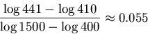
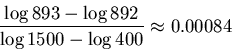
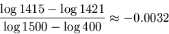
In terms of our example, an error of 1 for the mass
of ![]() , 441 would be equivalent to an error
of
, 441 would be equivalent to an error
of
![]() for
for ![]() for the mass 1415.
A standard transformation, when we want to linearize
relative values, is to use the logarithms of the
measures.
So instead of working with the weights, we will
work with the logarithms of the weights.
A tolerance of
for the mass 1415.
A standard transformation, when we want to linearize
relative values, is to use the logarithms of the
measures.
So instead of working with the weights, we will
work with the logarithms of the weights.
A tolerance of ![]() in the logarithms is
equivalent to a relative tolerance of
in the logarithms is
equivalent to a relative tolerance of
![]() in the relative values.
This is valid approximation for sufficiently small
in the relative values.
This is valid approximation for sufficiently small ![]() .
.
Finally, since our intervals in the theoretical derivation
were based on random variables distributed in (0,1),
we must make the relative errors relative to the size
of the entire interval, or divide them by
![]() where
where ![]() and
and ![]() are the
maximum and minimum weights that we will consider
in the sample.
are the
maximum and minimum weights that we will consider
in the sample.
In our example, ![]() and
and ![]() so the
radius of the error for
so the
radius of the error for ![]() is
is
We have now all the ingredients for our algorithm.
For each protein in the database we compute its
digestion in, say, ![]() fragments, and the weights
of these fragments.
For each searched weight
fragments, and the weights
of these fragments.
For each searched weight ![]() we find the minimum
distance to one of the database weights
we find the minimum
distance to one of the database weights ![]() and set
and set
![]() .
Then we order the distances in increasing values
.
Then we order the distances in increasing values
![]() .
For distance
.
For distance ![]() ,
, ![]() weights are within distance
weights are within distance ![]() of database weights.
For each
of database weights.
For each ![]() we compute
we compute ![]() .
The best match is considered the
.
The best match is considered the ![]() for which
for which ![]() is minimal.
This probability identifies the database sequence.
is minimal.
This probability identifies the database sequence.
![]() is
the score of the match with this database sequence.
Finally we keep track of the
is
the score of the match with this database sequence.
Finally we keep track of the ![]() lowest probabilities
or highest scores
(
lowest probabilities
or highest scores
(![]() usually between 5 and 20) for all sequences in the database.
usually between 5 and 20) for all sequences in the database.
This function will be called SearchMass and receives as parameters a set of weights, a function which does the digestion, as shown earlier with DigestTrypsin, and the value IT(m).
SearchMass := proc( weights:array(float), Digest:procedure,
        m:posint )
description 'Search the database for similar mass profiles';
if not type(DB,database) then
    error('a protein database must be loaded with ReadDb') fi;

# create the output array (with maximum probability entries)
BestMatches := CreateArray( 1..m, [1] );

# sort the input weights and compute weight bounds
w := sort(weights);
logw := zip(log(w));
lw := length(w);
wmax := w[lw] * 1.02;
wmin := w[1] * 0.98;
d := CreateArray( 1..lw );
IntLen := log(wmax) - log(wmin);

# for each sequence in the database do the digestion
# and compute the weights
for s in Sequences() do
    v := sort(GetMolWeight(Digest(s)));
    logv := zip(log(v));

    # compute the d_i values
    j := 0;
    lv := length(v);
    for i to lw do
	# compute all the differences for w[i]
	diffs := { seq( |logw[i]-j|, j=logv )};
	d[i] := 2*diffs[1] / IntLen;
    od;

    # compute n, the number of weights between wmax and wmin
    n := 0;
    for j to lv do
        if v[j] >= wmin and v[j] <= wmax then n := n+1 fi od;
    if n < 2 then next fi;

    # sort the interval widths and compute the most rare event
    d := sort(d);
    p := 1;
    for k to lw do
        if d[k] > 0 then
            pk := ( 1 - exp(-n*d[k]) ) ^ k;
            if pk < p then kmin := k;  p := pk fi
        fi
    od;
Instead of working with probabilities directly, we will work with the logarithm of these probabilities. To make these measures similar to the similarity scores of alignments, we will compute -10 log10 p. This measure will now be comparable to scores obtained from alignments using the standard Dayhoff matrices.
    sim := -10 * log10(p);
    if sim > BestMatches[1,1] then
	# new smallest probability found, insert and reorder
        BestMatches[1] := [sim,GetEntryNumber(s),n,kmin];
        BestMatches := sort( BestMatches, x -> x[1] );
    fi
od;
BestMatches
end:
The above function is implemented in Darwin's kernel with additional generality. The main reason for having it in the kernel is to compute faster. The kernel function is also able to handle DNA searching, many predefined digestors and changes to the molecular weight of amino acids. It is useful to see its description and to see the list of digestors supported.
?SearchMassDb
Function SearchMassDb - Searches digestion fragments against a database
Option: builtin

Calling Sequence:  SearchMassDb(p,n)

Parameters:
  Name   Type      Description
  ----------------------------------------------------------------
  p      Protein   description of protein (weights, enzymes, etc.)
  n      integer   maximum number of returned matches

Returns:
	MassProfileResults
Synopsis:  Searches the n most significant matches of weights of digested
  fragments. The search is done against the database which is currently loaded
  (with the command ReadDb).  This could be a protein or a nucleotide
  database.  The description of the protein to be searched is in terms of the
  (one or many) weights resulting from digesting the protein with an enzyme.
  This description can also hold other information as deuteration, and
  modified amino acid weights.  See Protein and DigestionWeights for details.
  The result is a data structure which contains the best n matches, ordered
  from best to worst.  Each match is described by the similarity score, number
  of fragments in the protein, number of matched fragments, and description of
  the matching protein.  See MassProfileResults for full details.

Examples:
> DB := ReadDb('/home/darwin/DB/SwissProt.Z'):;
Peptide file(/home/darwin/DB/SP45.0/SwissProt45.0(169638448), 163235
 entries, 59631787 aminoacids)
> print( SearchMassDb( Protein(DigestionWeights('Trypsin',
    601.9438, 504.0904, 1512.4545, 480, 590)), 5 ));


Score  n k   AC      DE		   OS
 60.4 21 4 P28519;  DNA repair protein RAD14.  Saccharomyces cerevisiae
                    (Baker's yeast). Unmatched weights: [1512.5].
 60.0  7 3 Q43284;  Oleosin 14.9 kDa.  Arabidopsis thaliana (Mouse-ear cress).
                    Unmatched weights: [480.0, 1512.5].
 59.8 17 4 P21908;  Glucokinase (EC 2.7.1.2) (Glucose kinase).  Zymomonas
                    mobilis. Unmatched weights: [590.0].
 58.2  6 3 Q9FC39;  Protein crcB homolog 1.  Streptomyces coelicolor.
                    Unmatched weights: [590.0, 1512.5].
 57.3 11 3 P06931;  E6 protein.  Bovine papillomavirus type 1. Unmatched
                    weights: [590.0, 601.9].
See Also:
           ?DigestAspN          ?DigestWeights    ?MassProfileResults
           ?DigestionWeights    ?DynProgMass      ?ProbBallsBoxes
           ?DigestSeq           ?DynProgMassDb    ?ProbCloseMatches
           ?DigestTrypsin       ?enzymes


   ------------
?enzymes
For SearchMassDb the following enzymes are recognized (courtesy
of Amos Bairoch):

 Enzyme name		cuts between			except for
 ###########		############			##########

 Armillaria		Xaa-Cys,Xaa-Lys
 ArmillariaMellea	Xaa-Lys
 BNPS_NCS		Trp-Xaa
 Chymotrypsin		Trp-Xaa,Phe-Xaa,Tyr-Xaa,	Trp-Pro,Phe-Pro,Tyr-Pro,
			Met-Xaa,Leu-Xaa,		Met-Pro,Leu-Pro
 Clostripain		Arg-Xaa
 CNBr_Cys		Met-Xaa,Xaa-Cys
 CNBr			Met-Xaa
 AspN			Xaa-Asp
 LysC			Lys-Xaa
 Hydroxylamine		Asn-Gly
 MildAcidHydrolysis	Asp-Pro
 NBS_long		Trp-Xaa,Tyr-Xaa,His-Xaa
 NBS_short		Trp-Xaa,Tyr-Xaa
 NTCB			Xaa-Cys
 PancreaticElastase	Ala-Xaa,Gly-Xaa,Ser-Xaa,Val-Xaa
 PapayaProteinaseIV	Gly-Xaa
 PostProline		Pro-Xaa				Pro-Pro
 Thermolysin		Xaa-Leu,Xaa-Ile,Xaa-Met,
			Xaa-Phe,Xaa-Trp,Xaa-Val
 TrypsinArgBlocked	Lys-Xaa				Lys-Pro
 TrypsinCysModified	Arg-Xaa,Lys-Xaa,Cys-Xaa		Arg-Pro,Lys-Pro,Cys-Pro
 TrypsinLysBlocked	Arg-Xaa				Arg-Pro
 Trypsin		Arg-Xaa,Lys-Xaa			Lys-Pro
 V8AmmoniumAcetate	Glu-Xaa				Glu-Pro
 V8PhosphateBuffer	Asp-Xaa,Glu-Xaa			Asp-Pro,Glu-Pro

The following are double digestors (both acting simultaneously)
 CNBrTrypsin            Met-Xaa
                        Arg-Xaa,Lys-Xaa                 Lys-Pro
 CNBrAspN               Met-Xaa
                        Xaa-Asp
 CNBrLysC               Met-Xaa
                        Lys-Xaa
 CNBrV8AmmoniumAcetate  Met-Xaa
                        Glu-Xaa                         Glu-Pro
 CNBrV8PhosphateBuffer  Met-Xaa
                        Asp-Xaa,Glu-Xaa                 Asp-Pro,Glu-Pro

Comments:
 CNBr_Cys - its chemistry is not well defined so modifications of
	other amino acids may occur.

 NBS_log
 NBS_short
 NTCB
 BNPS_NCS - these four digesters produce unpredictable chemical modifications
	of other residues which will adversely affect the search.

  Hydroxylamine
  MildAcidHydrolysis - both of these produce at most one or two fragments per
	protein and are therefore not useful for searching.

  Chymotrypsin
  PancreaticElastase
  Thermolysin - are not as specific (or go to completion) as it would be
	desired.

  PapayaProteinaseIV
  PostProline - these enzymes can only cleave small proteins, and hence are
	not of great practical use.

  CNBr - instead of methionine being left at the C-terminal, a homoserine
	(101.1054) or homoserine lactone (83.092) is produced.

  TrypsinCysModified - all the cysteines are transformed into aminoethyl-
	cysteine (146.2133).

   ------------
Suppose we are given the molecular weights:
ws := [ 511.3, 563.1, 717.2, 743.2, 836.4, 842.5, 1014.4,
	1169.4, 1387.5, 1509.7, 1524.0 ]:
dws := DigestionWeights( Trypsin, op(ws) ):
from the results of digesting an unknown protein with trypsin. DigestionWeights is a data structure which holds the results of a digestion with an enzyme. See ?DigestionWeights for details on how to express weight modifications. To compute the 5 most significant matches, after loading the database, we run the command
SwissProt := '/home/cbrg/DB/SwissProt.Z':
ReadDb(SwissProt);
Reading 169638448 characters from file /home/cbrg/DB/SwissProt.Z
Pre-processing input (peptides)
163235 sequences within 163235 entries considered
Peptide file(/home/cbrg/DB/SwissProt.Z(169638448), 163235 entries, 59631787
 aminoacids)
res := SearchMassDb( Protein(dws), 5 );
res := MassProfileResults([76.1635, 1773, 28, 5, [-1509.7000, -1387.5000,
-842.5000, -836.4000, -717.2000, -563.1000, 511.3000, 743.2000, 1014.4000,
1169.4000, 1524]],[76.5608, 40150, 10, 4, [-1509.7000, -1387.5000, -1014.4000,
-836.4000, -743.2000, -717.2000, -511.3000, 563.1000, 842.5000, 1169.4000, 1524]
],[82.2032, 121336, 12, 6, [-1524, -1509.7000, -1387.5000, -1014.4000,
-836.4000, 511.3000, 563.1000, 717.2000, 743.2000, 842.5000, 1169.4000]],[
83.5932, 40618, 24, 6, [-1509.7000, -1169.4000, -1014.4000, -836.4000,
-511.3000, 563.1000, 717.2000, 743.2000, 842.5000, 1387.5000, 1524]],[159.3941,
36958, 15, 9, [-563.1000, -511.3000, 717.2000, 743.2000, 836.4000, 842.5000,
1014.4000, 1169.4000, 1387.5000, 1509.7000, 1524]])
The result of SearchMassDb is a MassProfileResults structure. Each element of the structure represents a good hit and has 5 components: the similarity score, the entry number, the number of selected weights from the database (n) the number of matched weights from the sample (k) and a list with the database protein weights given, the matched ones positive and the unmatched ones as negative. We can print the results in a more readable format:
print(res);
Score  n k   AC      DE		   OS
159.4 15 9 P80049;  Fatty acid-binding protein, liver (L-FABP).  Ginglymostoma
                    cirratum (Nurse shark). Unmatched weights: [511.3, 563.1].
 83.6 24 6 Q9SJP6;  Putative fucosyltransferase 10 (EC 2.4.1.-) (AtFUT10)
                    (Fragment).  Arabidopsis thaliana (Mouse-ear cress).
                    Unmatched weights: [511.3, 836.4, 1014.4, 1169.4, 1509.7].
 82.2 12 6 Q9RH74; Q89K47;  SsrA-binding protein.  Bradyrhizobium japonicum.
                    Unmatched weights: [836.4, 1014.4, 1387.5, 1509.7, 1524.0].
 76.6 10 4 P75038;  Putative 1-phosphofructokinase (EC 2.7.1.56) (Fructose
                    1-phosphate kinase).  Mycoplasma pneumoniae. Unmatched
                    weights: [511.3, 717.2, 743.2, 836.4, 1014.4, 1387.5,
                    1509.7].
 76.2 28 5 P22966;  Angiotensin-converting enzyme, testis-specific isoform
                    precursor (EC 3.4.15.1) (ACE-T) (Dipeptidyl carboxypeptidase
                    I) (Kininase II).  Homo sapiens (Human). Unmatched weights:
                    [563.1, 717.2, 836.4, 842.5, 1387.5, 1509.7].
The above results are typical of a successful match (the top one representing a probability of 1e-16 of being so good by random chance) followed by matches which are in the noise area (probability of 1e-8 which is on the order of the size of the database, fewer weights matched and no consistent name of the matched protein.
How can we determine if the above similarities are significant or not? The scores are 10 times the log of probabilities, but these probabilities are for a single sequence of the database. How significant a match is against the entire protein database is much more complicated to evaluate. It would require to consider the total number of sequences and the total number of choices of fragments to match. The sequences in the database sometimes exhibit very high similarity and cannot be considered as independent. A Montecarlo method is much more appropriate to answer the significance question. We will run the search for various randomly generated sequences and tabulate their values. For this example we first generate as many random weights as we had in the sample, uniformly distributed in the same range,
wmin := min(ws) * 0.98; wmax := max(ws) * 1.02;
wmin := 501.0740
wmax := 1554.4800
set counters to collect statistics and run 10 database searches
ran := Stat('Random score'):  tim := Stat('Search time (secs)'):
to 10 do
    rw := [ seq( Rand(wmin..wmax), i=1..length(ws) )];
    st := time();
    res2 := SearchMassDb(Protein(DigestionWeights(Trypsin,op(rw))),1);
    UpdateStat(tim,time()-st);
    UpdateStat(ran,res2[1,1]);
od:
weights 1371.12 and 1372.37 are suspiciously close together
The results of this simulation are:
print(ran,tim);
 Random score: number of sample points=10
 mean = 88.1 +- 5.2
 variance = 71 +- 44
 skewness=-0.247997,   excess=-1.1077
 minimum=74.2442,     maximum=99.4162

 Search time (secs): number of sample points=10
 mean = 3.402 +- 0.076
 variance = 0.015 +- 0.015
 skewness=-1.20439,   excess=1.57675
 minimum=3.14,     maximum=3.53
Now we can state that for this database, similarity scores smaller than
ran[Mean] + 1.96*sqrt(ran[Variance]);
104.5630
are not very surprising or interesting (they happen for random weights, 2.5% of the time). Our most significant match in the previous example is
(res[5,1] - ran[Mean]) / sqrt(ran[Variance]);
8.4827
standard deviations away from the average, and this is very significant, if the distribution of a score based on random weights would be normal, it would happen with probability
erfc( "/sqrt(2) ) / 2;
1.1e-17
This value is in excellent agreement with the score of
159.3941. Hence we can conclude that the weights 511.3, 563.1, 717.2, etc. come from the digestion of the fatty acid-binding liver protein of sharks or similar sequences with a very high likelihood.Next we will show how two digestions of the same protein increase the confidence of our results. The procedure described above can be extended to use more than one digestion data. The kernel function accepts more than one digestion information. To test this we will:
| (i) | select a protein from the database, so that we know if we are successful or not in the search, |
| (ii) | digest it theoretically with two different enzymes, AspN and Trypsin, |
| (iii) | collect 2 weights of each digestion (a very minimal number) between 600 and 1500 daltons, |
| (iv) | add some noise to those weights, |
| (v) | add random weights to the search and |
| (vi) | search the database with the weights of the two digestions. |
# choose a particular sequence
s := Sequence(AC(P34010));
s := MFMYPEFARKALSKLISKKLNIEKVSSKHQLVLLDYGLHGLLPKSLYLEA ..(666).. SIILDDINGTR
# digest and select weights (use Darwin's general digestion function)
wsAspN := mselect( x -> x >= 600 and x <= 1500, DigestWeights(s,AspN) );
wsTryp := mselect( x -> x >= 600 and x <= 1500, DigestWeights(s,Trypsin) );
Warning: procedure DigestTrypsin reassigned
wsAspN := [1345.5330, 1056.2590, 1083.1280, 788.9260, 1307.4540, 945.0250,
696.7890, 1360.4570, 920.0580, 752.7650, 1371.5000, 674.6980]
wsTryp := [1191.4200, 615.7140, 790.8840, 765.8220, 816.9160, 1244.4040,
707.8480, 1113.3260, 1485.6880, 1081.2620, 854.9810, 908.9850, 1201.3690,
910.9720, 781.9510, 1021.1450, 602.7410, 931.9460, 721.8410, 799.9390, 1034.2280
, 602.8050, 1006.2170, 1491.7160, 811.9340, 938.9930, 1024.1520, 887.0300,
1305.4190, 779.8720, 715.7910, 1055.1900, 1107.3430, 1491.6900, 1348.5900,
1245.4300, 642.7660, 1371.5000]
Darwin issues a warning when a procedure is reassigned. The procedure DigestTrypsin was assigned at the beginning of this biorecipe. Calling DigestWeights here forces reading of the entire set of functions related to molecular weight including the library version of DigestTrypsin. Thus it is reassigned and a warning is issued.
# select two arbitrary weights and perturb with random error
wsAspN := wsAspN[3]+Rand(-0.1..0.1), wsAspN[6]+Rand(-0.1..0.1);
wsTryp := wsTryp[3]+Rand(-0.1..0.1), wsTryp[6]+Rand(-0.1..0.1);
wsAspN := 1083.1723, 944.9278
wsTryp := 790.9820, 1244.4106
# add random weights
ws1 := DigestionWeights( AspN, wsAspN, seq( Rand(600..1500), i=1..4 ) );
ws2 := DigestionWeights( Trypsin, wsTryp, seq( Rand(600..1500), i=1..5 ) );
ws1 := DigestionWeights(AspN,1083.1723,944.9278,817,1475,767,726)
ws2 := DigestionWeights(Trypsin,790.9820,1244.4106,1373,1212,1166,1322,675)
# search database and print results
print( SearchMassDb( Protein(ws1, ws2), 5 ) ):
Score  n k  n k   AC      DE		   OS
103.1 15 3 18 4 P59107;  Exoribonuclease II (EC 3.1.13.1) (Ribonuclease II)
                         (RNase II).  Shigella flexneri. Unmatched weights:
                         [726.0, 767.0, 1475.0]. Unmatched weights: [791.0,
                         1322.0, 1373.0].
102.8  7 3 16 5 O60663; O75463;  LIM homeobox transcription factor 1 beta (LIM/
                         homeobox protein LMX1B) (LIM-homeobox protein 1.2)
                         (LMX-1.2).  Homo sapiens (Human). Unmatched weights:
                         [767.0, 944.9, 1083.2, 1475.0]. Unmatched weights:
                         [1166.0, 1373.0].
 99.7 11 2 31 2 P34010;  Protein O1.  Variola virus. Unmatched weights: [726.0,
                         767.0, 817.0, 1475.0]. Unmatched weights: [675.0,
                         1166.0, 1212.0, 1322.0, 1373.0].
 98.5  6 2 10 3 P35502;  Esterase FE4 precursor (EC 3.1.1.1) (Carboxylic-ester
                         hydrolase).  Myzus persicae (Peach-potato aphid).
                         Unmatched weights: [726.0, 767.0, 817.0, 944.9].
                         Unmatched weights: [791.0, 1166.0, 1244.4, 1373.0].
 93.4  6 1 16 5 O88609;  LIM homeobox transcription factor 1 beta (LIM/homeobox
                         protein LMX1B) (LIM-homeobox protein 1.2) (LMX-1.2).
                         Mus musculus (Mouse). Unmatched weights: [726.0, 767.0,
                         944.9, 1083.2, 1475.0]. Unmatched weights: [1166.0,
                         1373.0].
We can see that the desired protein was found, although due to the small number of matching weights, noise and additional weights, the match is at the same level as the other irrelevant matches. This was made a limiting case on purpose, to show what happens when the weight information is barely enough. If we would repeat this experiment with at least one more matching weight, the results would be unambiguous.
This last case is very interesting, since the lab procedures to extract protein samples, (e.g. 2D electrophoresis) cannot guarantee that we isolate a single protein. Often, one spot may have two superimposed proteins. Hence it is important to see if having enough weight information discovers the multiple proteins. As above, we will use a limiting case to show the minimal amount of information that will detect the proteins. To test this we will:
| (i) | select two proteins from the database, so that we know if we are successful or not in the search, |
| (ii) | digest them theoretically with Trypsin, |
| (iii) | collect 3 weights of each protein between 600 and 1500 daltons, |
| (iv) | add some noise to those weights, |
| (v) | add random weights to the search and |
| (vi) | search the database with the weights. |
# choose two particular sequences
s1 := Sequence(AC(Q9WX16));
s2 := Sequence(AC(Q06650));
s1 := MTEKALRLGTRRSKLAMAQSGQVADAVSQVTGRPVELVEITTYGDTSREH ..(319).. GAAGLMGERAQ
s2 := MRKPTSSLTRRSVLGAGLGLGGALALGSTTASAASAGTTPSENPAAVRRL ..(311).. ATVLSEAVAPA
# digest and select weights (use Darwin's general digestion function)
ws1 := mselect( x -> x >= 600 and x <= 1500, DigestWeights(s1,Trypsin) );
ws2 := mselect( x -> x >= 600 and x <= 1500, DigestWeights(s2,Trypsin) );
ws1 := [1201.2930, 657.6950, 713.8190, 656.7060, 1037.1880, 1382.5720, 660.6510,
606.6830, 716.7590]
ws2 := [889.0050, 639.6560, 1408.6750, 885.0420, 1226.2570, 925.9510, 795.8600,
1158.2880, 906.0140, 1352.5150, 1000.0870, 843.9020, 1428.4660, 1195.2750,
969.1200, 1100.3140, 1054.1540, 775.8250, 969.9430, 1141.2780]
# select 3 arbitrary weights from each and perturb with error
ws := seq( ws1[i]+Rand(-0.1..0.1), i=[2,4,6,7] ),
      seq( ws2[i]+Rand(-0.1..0.1), i=[3,6,7,9] );
ws := 657.7264, 656.7512, 1382.5456, 660.6899, 1408.6820, 925.9595, 795.8261,
906.0139
# add random weights
ws := DigestionWeights( Trypsin, ws, seq( Rand(600..1500), i=1..3 ) );
ws := DigestionWeights(Trypsin,657.7264,656.7512,1382.5456,660.6899,1408.6820,
925.9595,795.8261,906.0139,1355,1153,1220)
# search database and print results
print( SearchMassDb( Protein(ws), 5 ) ):
Score  n k   AC      DE		   OS
122.3  8 4 Q9WX16;  Porphobilinogen deaminase 1 (EC 2.5.1.61) (PBG 1)
                    (Hydroxymethylbilane synthase 1) (HMBS 1) (Pre-
                    uroporphyrinogen synthase 1).  Streptomyces coelicolor.
                    Unmatched weights: [795.8, 906.0, 926.0, 1153.0, 1220.0,
                    1355.0, 1408.7].
108.9 19 4 Q06650;  Beta-lactamase precursor (EC 3.5.2.6) (Penicillinase).
                    Streptomyces cellulosae. Unmatched weights: [656.8, 657.7,
                    660.7, 1153.0, 1220.0, 1355.0, 1382.5].
 98.4 16 4 Q07523;  Hydroxyacid oxidase 3 (EC 1.1.3.15) (HAOX3) ((S)-2-hydroxy-
                    acid oxidase, peroxisomal) (Long chain alpha-hydroxy acid
                    oxidase) (Long- chain L-2-hydroxy acid oxidase).  Rattus
                    norvegicus (Rat). Unmatched weights: [656.8, 657.7, 795.8,
                    926.0, 1153.0, 1220.0, 1355.0].
 91.6 97 5 Q61043; Q6ZPM7;  Ninein.  Mus musculus (Mouse). Unmatched weights:
                    [656.8, 906.0, 1153.0, 1220.0, 1355.0, 1408.7].
 89.8 57 4 P10220;  Large tegument protein (Virion protein UL36).  Human
                    herpesvirus 1 (strain 17) (HHV-1) (Human herpes simplex
                    virus 1). Unmatched weights: [656.8, 660.7, 926.0, 1153.0,
                    1220.0, 1355.0, 1408.7].
We can see both desired proteins were found with the scores better than the other matches although the score of the second match is approaching the noise area.
© 2009 by Gaston Gonnet Gina Cannarozzi, Informatik, ETH Zurich
Please cite as:
@techreport{ Gonnet-TPI,
        author = {Gaston H. Gonnet, Gina M. Cannarozzi},
        title = {Recognizing Proteins by Weight of their Digested Parts},
        month = { },
        year = {},
        number = { },
        howpublished = { Electronic publication },
        copyright = {code under the GNU General Public License},
        institution = {Informatik, ETH, Zurich},
        URL = { http://www.biorecipes.com/MolWeight/code.html }
        }
Last updated on Fri Mar 27 11:30:35 2009 by GMC