In this bio-recipe we will analyze how significant is an alignment. This will be done by comparing the real alignment against alignments made out of shufflings of the same sequences.
First we define the file name where we can find the SwissProt database and then load it. We also create Dayhoff matrices to be able to align sequences.
SwissProt := '/home/cbrg/DB/SwissProt.Z':
ReadDb(SwissProt);
CreateDayMatrices();
Reading 169638448 characters from file /home/cbrg/DB/SwissProt.Z
Pre-processing input (peptides)
163235 sequences within 163235 entries considered
Peptide file(/home/cbrg/DB/SwissProt.Z(169638448), 163235 entries, 59631787
 aminoacids)
Given two sequences from the database (given by the accession numbers)
seq1 := Sequence(AC(P58051));
seq2 := Sequence(AC(Q64403));
seq1 := MIWWFIVGASFFFAFILIAKDTRTTKKNLPPGPPRLPIIGNLHQLGSKPQ ..(496).. LQLIPVLTQWT
seq2 := MGLLTGDALFSVAVAVAIFLLLVDLMHRRQRWAARYPPGPVPVPGLGNLL ..(500).. PSPYQLCAVLR
We align the two sequences using a local alignment, to align the best subsequences.
al1 := Align(seq1,seq2,Local);
al1 := Alignment(Sequence(AC('P58051'))[2..464],Sequence(AC('Q64403'))[9..474],376.1353,DM,0,0,{Local})
The alignment printed in a readable format is:
print(al1);
lengths=463,466 simil=376.1, PAM_dist=250, identity=23.3%
ID=C72E_ARATH   AC=P58051;   DE=Cytochrome P450 71B14 (EC 1.14.-.-).
OS=Arabidopsis thaliana (Mouse-ear cress).   OC=Eukaryota; Viridiplantae;
Streptophyta; Embryophyta; Tracheophyta; Spermatophyta; Magnoliophyta;
eudicotyledons; core eudicots; rosids; eurosids II; Brassicales; Brassicaceae;
Arabidopsis.   KW=Heme; Monooxygenase; Multigene family; Oxidoreductase;
Transmembrane.
ID=CPDG_CAVPO   AC=Q64403; O54866;   DE=Cytochrome P450 2D16 (EC 1.14.14.1)
(CYPIID16).   OS=Cavia porcellus (Guinea pig).   OC=Eukaryota; Metazoa;
Chordata; Craniata; Vertebrata; Euteleostomi; Mammalia; Eutheria; Rodentia;
Hystricognathi; Caviidae; Cavia.   KW=Direct protein sequencing; Electron
transport; Endoplasmic reticulum; Heme; Membrane; Microsome; Monooxygenase;
Oxidoreductase.
IWWFIVGASFFFAFILIAKDTRTTKKNLPPGPPRLPIIGNLHQLG_SKPQRSLFKLSEKYGSLMSLKFGNVSAVVASTPE
!! :.|::::|:.:! !.:..:. ..:.||||..:| !|||.|:: ::...|. ||.::!|:::||:|  :::||::..
LFSVAVAVAIFLLLVDLMHRRQRWAARYPPGPVPVPGLGNLLQVDFENMAYSCDKLRHQFGDVFSLQFVWTPVVVVNGLL

TVKDVLKTFDAECCSRPYMTYPARVTYNFNDLAF__SPYSKYWREVRKMTVIELYT_AKRVKSFQNVRQEEVASFVDFIK
:|!!:|.: ::!.::||.!:..|.:.!: :..::  : |:..|||.|!::|.:|.: :...||::: .:||:|::...::
AVREALVNNSTDTSDRPTLPTNALLGFGPKAQGVIGAYYGPAWREQRRFSVSSLRNFGLGKKSLEQWVTEEAACLCAAFT

QHASLEKTVNMKQKLVKLSGSVICKVGFGISLEWS_____KLANTYEEVIQGTMEVVGRFAAADYFPIIGRIIDRITGLH
:||:  :::..|..|.|...:||::: !:..:!!:     !|.:..||:!:.:.::  !:.:.:.:|!! ||  ..:.:.
NHAG__QPFCPKALLNKAVCNVISSLIYARRFDYDDPMVLRLLEFLEETLRENSSL__KIQVLNSIPLLLRIPCVAAKVL

SKCEKVFKEMDSFFDQSIKHHLEDTNIKDDIIGLLLKMEKGETGLGEFQLTRNHTKGILLNVLIAGVDTSGHTVTWVMTH
|..::::. .|:::.:. :....|:. !| . ::|.:|:|:: | :| :::.::.! !:.::: ||: |::.|::|:!..
SAQRSFIALNDKLLAEHNTGWAPDQPPRDLTDAFLTEMHKAQ_GNSESSFNDENLRLLVSDLFGAGMVTTSVTLSWALLL

LIKNPRVMKKAQAEVREVIKNKDDITEEDIERLEYLKMVIKETLRINPLVPLLIPREASKYIKIGGYDIPKKTWIYVNIW
!|.:|.|.!::|.|!.|||.:..  ...|..:!.!.:.||:|:.|:..!||! !|:.:|! .:!.|! |||.|.!!:|!
MILHPDVQRHVQEEIDEVIGQVRCPEMADQAHMPFTNAVIHEVQRFADIVPMGVPHMTSRDTEVQGFLIPKGTMLFTNLS

AVQRNPNVWKDPEVFIPERFMHSEIDYKGVDFELLPFGSGRRMCPGMGLGMALVHLTLINLLYRFDWKLPEG
:|.!:.:||::| .|.|.:|!::| .!...! .:!||::|.|:|.|..|:.. :.|.:.:||.||:!::|||
SVLKDETVWEKPLHFHPGHFLDAEGRFVKRE_AFMPFSAGPRICLGEPLARMELFLFFTSLLQRFSFSVPEG
Then we shuffle randomly the amino acids of both sequences and align them again. We repeat the random shuffling and alignment many times, so that we can have some reliable values for the average score. First we would like to have some information about how to shuffle sequences.
?Shuffle
the following help files contain (approximately) the keyword:
  ?Beta_Rand
  ?Binomial_Rand
  ?ChiSquare_Rand
  ?Exponential_Rand
  ?FDist_Rand
  ?GammaDist_Rand
  ?Geometric_Rand
   ------------
The code to compute 400 random alignments and gather the statistics of its score is:
s := Stat('random score of shuffled seq1 and seq2'):
to 400 do
    a := Align(Shuffle(seq1),Shuffle(seq2),Global);
    s+a[Score]
    od:
This code uses the variable s
which is assigned a structure to collect univariate statistics.
Now we can print the results onto the screen
(in plain characters), or we can see them as a web page
(other possibilities, like Latex are also possible).
print(s);
 random score of shuffled seq1 and seq2: number of sample points=400
 mean = -135.6 +- 2.3
 variance = 531 +- 78
 skewness=0.43412,   excess=0.246474
 minimum=-191.574,     maximum=-54.6842
View(HTML(s));
<?xml version="1.0" encoding="utf-8" ?>
<!DOCTYPE html PUBLIC "-//W3C//DTD XHTML 1.0 Transitional//EN"
    "http://www.w3.org/TR/xhtml1/DTD/xhtml1-transitional.dtd">
<html xmlns="http://www.w3.org/1999/xhtml">
     <head>
<!-- automatically generated by Darwin
prepared on Mon Oct 24 17:21:44 CEST 2011
running on linneus75
by user darwin
-->
</head><body BGCOLOR="#E0E0E0">
<TABLE ALIGN=CENTER BORDER CELLSPACING=5 BGCOLOR="C0C0C0">
<CAPTION ALIGN=BOTTOM>random score of shuffled seq1 and seq2</CAPTION>
<TR> <TH>sample size</TH>
<TH>mean</TH> <TH>variance</TH> <TH>skewness</TH> <TH>excess</TH>
<TH>minimum</TH> <TH>maximum</TH> </TR>
<TR> <TD ALIGN=CENTER>400</TD><TD ALIGN=CENTER>-135.6±2.3</TD><TD ALIGN=CENTER>531±78</TD><TD ALIGN=CENTER>0.4341</TD><TD ALIGN=CENTER>0.2465</TD><TD ALIGN=CENTER>-191.6</TD><TD ALIGN=CENTER>-54.68</TD>
</TABLE>
</body></html>
Global alignments are really poor (forcing the entire shuffled entries to match), so we may try Local alignments, that is the best subsequences that match. At this point we also want to create a histogram of the scores, to have a visual clue on their distribution.
Hist := CreateArray(1..100):
s2 := Stat('random (Local) score of seq1 and seq2'):
to 800 do
    a := Align(Shuffle(seq1),Shuffle(seq2),Local);
    s2+a[Score];
    i := round(a[Score]);
    Hist[i] := Hist[i]+1;
    od:
print(s2);
 random (Local) score of seq1 and seq2: number of sample points=800
 mean = 46.39 +- 0.38
 variance = 30.6 +- 4.1
 skewness=0.970446,   excess=1.74417
 minimum=36.2973,     maximum=74.8547
The histogram, which is produced as a postscript file, can be viewed on a separate window.
View(Histogram(Hist));
If we want to focus the histogram on the part where all the significant scores happen, we select the values between 35 and 80.
View(Histogram(Hist[35..80]));
We see from the histogram, that although the distribution is skewed to the right, it is pretty much normal-shaped. Assuming that the scores are normal distributed and given that the original score was around 376, and that the average of a random score is about 46 with a variance of 31, the hypothesis that the original score could be obtained at random is extremely unlikely. The following expression computes how many standard deviations away it is from the average:
(al1[Score]-s2[Mean]) / sqrt(s2[Variance]);
59.5698
This corresponds to a p-value which is smaller than 10^-400 and thus can non longer be represented using IEEE floating point representation.
On the other hand, from theory we know that alignment scores of random strings should follow the Gumbel distribution. Its cumulative is
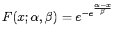
One possibility to estimate the necessary parameters according to our data is, to match the first two modes, i.e. the mean and standard deviation. They are given by


where gamma is the Euler-Mascheroni constant which is approximately 0.5772156. Of course, this way of estimating the parameters is far from optimal, but for the purpose of this exercise it is good enough. Thus,
beta := sqrt( s2[Variance]*6 ) / Pi;
alpha := s2[Mean]-0.5772156*beta;
beta := 4.3159
alpha := 43.9020
Let us now compare the histogram to the two distributions in question:
normal := x->1/sqrt(2*Pi*s2[Variance])*exp( -(x-s2[Mean])^2/(2*s2[Variance]));
gumbel := x->exp((alpha-x)/beta)/beta * exp(-(exp((alpha-x)/beta)));
data := x->Hist[ round(x) ]/sum(Hist);
StartOverlayPlot();
DrawPlot(data, 30..80);
DrawPlot(normal, 30..80);
DrawPlot(gumbel, 30..80);
StopOverlayPlot();
View();
normal := x -> sqrt(2*Pi*s2[Variance])^(-1)*exp(-1*(x-1*s2[Mean])^2/(2*s2[
Variance]))
gumbel := x -> exp((alpha-1*x)/beta)/beta*exp(-1*exp((alpha-1*x)/beta))
data := x -> Hist[round(x)]/sum(Hist)
Warning: procedure DrawPlot reassigned
1
2
3
Warning: procedure DrawPlot reassigned

By visual inspection, we realize that the Gumbel distribution fits our data much better. Finally, we can also estimate the p-value with respect to the Gumbel distribution of our initial alignment.
pval := -expx1( -exp( (alpha-al1[Score])/beta) );
pval := 3.7042e-34
Note that we made use of the expx1 function. This function computes exp(x)-1 and is numerically much more stable for x close to 0.
And the final conclusion is quite clear, a random alignment would never have the score that we obtained, nor anything close. The reason for the high score lies in the homology of the sequences.
© 2011 by Gaston Gonnet, Informatik, ETH Zurich
Last updated on Mon Oct 24 17:21:47 2011 by GhG
!!! This document is stored in the ETH Web archive and is no longer maintained !!!