This bio-recipe shows how to select random alignments to study certain properties in a way that the sample is not biased by the peculiar distribution of sequences in the database. We will then use this technique to sample alignments in a particular PAM distance range and study the distribution of gap lengths. The distribution of gap lengths is found to be Zipfian and this leads to a new deletion cost formula based on a logarithmic approximation. The discussion of alignments based on a logarithmic deletion cost is done in another bio-recipe with that subject.
First, lets understand what is wrong with finding alignments just by taking pairs of randomly selected sequences until we satisfy some criteria. The main problem biasing this method is the existence of many very close homologues in the database. Suppose that we find an interesting alignment between sequences A and B and another one between sequences C and D. Suppose that neither A nor B have close homologues, but C has 9 very close homologues and D has also 9 very close homologues. It is clear now that the alignment of C and D is going to be overrepresented in any random sample. First it is 100 times more likely to be selected at random. Secondly, if the sample is large, it is likely to be represented more than once. The purpose of the first part of this bio-recipe is to build a sample of alignments free from this bias. If you want to follow it, you might have to install the SwissProt data file which can be downloaded here.
We need a protein database so we define the location of the SwissProt database and then load it. We also create Dayhoff matrices to be able to align sequences.
SwissProt := 'SampleAlignments/SwissProt.Z':
ReadDb(SwissProt);
CreateDayMatrices();
Reading 169638448 characters from file SampleAlignments/SwissProt.Z
Pre-processing input (peptides)
163235 sequences within 163235 entries considered
Building new Pat index in file SampleAlignments/SwissProt.tree with 59631787 entries
Pat index with 59631787 entries
 sorted, from "A</SEQ></E>\n<E><ID>" to "YYYYYYYYYYYYGMSSIIF"
Peptide file(SampleAlignments/SwissProt.Z(169638448), 163235 entries, 59631787
 aminoacids)
First we initialize several variables. The set where we will store the candidate sequences to be compared Cand , the set of good Alignments found so far SampleAl and the limits of significance and PAM values to the selected alignments
Cand := SampleAl := {}:
minSim := 150:
loPAM := 40:
hiPAM := 80:
We will run the loop until we collect the desired number of alignments (in this case just one to make the bio-recipe run faster).
while length(SampleAl) < 1 do
   e := Rand(Entry);
   s := Sequence(e);
   if length(s) < 80 or length(s) > 900 then next fi;
Select a random Entry, and discard it its length is not between 80 and 900. Sequences too short or too long are unlikely to be desirable for this purpose. Now test the new sequence against all the ones which were selected before.
   tooClose := false:  possible := {}:
   for c in Cand do
      al := Align(Sequence(c),s);
      if al[Score] > minSim then
	  al := Align(al[Seq1],al[Seq2],DMS);
	  if al[PamDistance] < loPAM then
	       tooClose := true;  break
	  elif al[PamDistance] <= hiPAM then
	       possible := append(possible,al) fi
	  fi
      od;
If the new sequence is too close to an existing sequence, then discard it, else add any alignments that it could have contributed.
   if not tooClose then
	SampleAl := SampleAl union possible;
        Cand := append(Cand,e);
        fi:
   od:
length(Cand), length(SampleAl);
128, 1
The above loop will take considerable time to collect hundreds of matches, so for the purpose of this bio-recipe we will read a file which has been prepared exactly as above but with many more alignments.
ReadProgram( '/home/darwin/Repositories/teaching/bio-recipes/SampleAlignments/data.drw' );
length(SampleAl);
333
And we see that we have 333 alignments. All these alignments, because of the proximity restriction of the sequences, are essentially independent. We print one as a sample.
print(SampleAl[5]);
lengths=539,545 simil=2064.3, PAM_dist=71, identity=48.7%
ID=CH60_STRA3   AC=Q8CX22;   DE=60 kDa chaperonin (Protein Cpn60) (groEL
protein).   OS=Streptococcus agalactiae (serotype III).   OC=Bacteria;
Firmicutes; Lactobacillales; Streptococcaceae; Streptococcus.   KW=ATP-binding;
Chaperone; Complete proteome.
ID=HS60_SCHPO   AC=Q09864; Q10285;   DE=Heat shock protein 60, mitochondrial
precursor (HSP60).   OS=Schizosaccharomyces pombe (Fission yeast).
OC=Eukaryota; Fungi; Ascomycota; Schizosaccharomycetes; Schizosaccharomycetales;
Schizosaccharomycetaceae; Schizosaccharomyces.   KW=ATP-binding; Chaperone; Heat
shock; Mitochondrion; Transit peptide.
AKDIKFSADARSAMVRGVDILADTVKVTLGPKGRNVVLEKAFGSPLITNDGVTIAKEIELEDHFENMGAKLVSEVASKTN
|||:||..|||::!:.|||.||..|.||||||||||::!:.||||.||.||||!|!.!.|:|.|||!||!||.!||||||
AKDLKFGVDARASLLTGVDTLARAVSVTLGPKGRNVLIDQPFGSPKITKDGVTVARSVSLKDKFENLGARLVQDVASKTN

DIAGDGTTTATVLTQAIVREGLKNVTAGANPIGIRRGIETAVSAAVEELKEIAQPVSGKEAIAQVAAVSSRSE_KVGEYI
!!||||||||||||:||..|.:!||.||.||:.:||||:.||...|| |:. .:.!!..|.|:|||.!|:..! .!||.:
EVAGDGTTTATVLTRAIFSETVRNVAAGCNPMDLRRGIQLAVDNVVEFLQANKRDITTSEEISQVATISANGDTHIGELL

SEAMGRVGNDGVITIEESRGMETELEVVEGMQFDRGYLSQYMVTDNEKMVSELENPYILITDKKISNIQEILPLLEEVLK
::||.|||.!||||!:|.|.:..||||.|||:|||||:|.|:!|| :....|:|||.||:!!||!|.!|!||| || ..:
AKAMERVGKEGVITVKEGRTISDELEVTEGMKFDRGYISPYFITDVKSQKVEFENPLILLSEKKVSAVQDILPSLELAAQ

TNRPLLIIADDVDGEALPTLVLNKIRGTFNVVAVKAPGFGDRRKAMLEDIAILTGGTVVTEDLGLDLKDATMQVLGQSAK
..|||:|||!|||||||...!|||:||.:.|||!|||||||.|!.||.|:|!||...|..!!:.:.::.|. : ||....
QRRPLVIIAEDVDGEALAACILNKLRGQLQVVAIKAPGFGDNRRNMLGDLAVLTDSAVFNDEIDVSIEKAQPHHLGSCGS

VTVDKDSTVIVEGAGDSSAIANRVAIIKSQM_EATTSDFDREKLQERLAKLAGGVAVIKVGAATETELKEMKLRIEDALN
|||.|!.|!|.:||||...!.:|...|!..| !...!!!!!||||||||||:||!||||||.:!|.|:.|.| ||.||||
VTVTKEDTIIMKGAGDHVKVNDRCEQIRGVMADPNLTEYEKEKLQERLAKLSGGIAVIKVGGSSEVEVNEKKDRIVDALN

ATRAAVEEGIVSGGGTALVNVIEKVAALKL______NGDEETGRNIVLRALEEPVRQIAYNAGYEGSVIIERLKQ___SE
|.!|||.||!:.|.||::|.     |:|!|      | |::.|..||.!|:..|.:.|. |||.||::|!.!||:   .|
AVKAAVSEGVLPGAGTSFVK_____ASLRLGDIPTNNFDQKLGVEIVRKAITRPAQTILENAGLEGNLIVGKLKELYGKE

IGTGFNAANGEWVDMVTTGIIDPVKVTRSALQNAASVASLILTTEAVVANKPEPEAPTAPAMDPSM__MGGF
...|!:.|...:||! ..|!:||:||.|!.|.:|:.||||: |||..!.:  .||...||| .|.|  |||:
FNIGYDIAKDRFVDLNEIGVLDPLKVVRTGLVDASGVASLMGTTECAIVD__APEESKAPAGPPGMGGMGGM
We will now study the distribution of the gap lengths in these alignments. This is almost exactly the procedure followed in the paper by Gaston. H. Gonnet, Mark A. Cohen, and Steven A. Benner. "Empirical and structural models for insertions and deletions in the divergent evolution of proteins". Journal of Molecular Biology, 229:1065-1082, 1993. This paper shows that the distribution of the gap length is Zipfian. A Zipfian probability distribution follows:
                 1
     Pr[i] = ----------
              t
             i  Zeta(t)
where t>1 is a parameter of the distribution and Zeta(t) is needed to normalize the probabilities so that they add to one.
The next computational task is to collect the gap lengths. We will take from each sequence in each alignment the gaps and tally the number of occurrences per gap length. This is done with the following statements.
G := CreateArray(1..50):
for al in SampleAl do
   dps := DynProgStrings(al);
   for s in [ dps[2], dps[3] ] do
      while length(s) > 0 do
To find each gap we search for the first underscore and then count how many there are. Notice the operations on text shifting, done by adding an integer to a text (left addition shifts the left end, right addition shifts the right end).
	i := SearchString( '_', s );
	 if i<0 then break fi;
	 s := i+s;
	 for i to length(s)-1 while s[i+1]='_' do od;
	 s := i+s;
	 if i <= length(G) then G[i] := G[i] + 1 fi
         od
      od
   od:
G[1..20];
[438, 142, 82, 54, 54, 20, 22, 18, 11, 9, 9, 8, 6, 7, 6, 3, 2, 0, 1, 2]
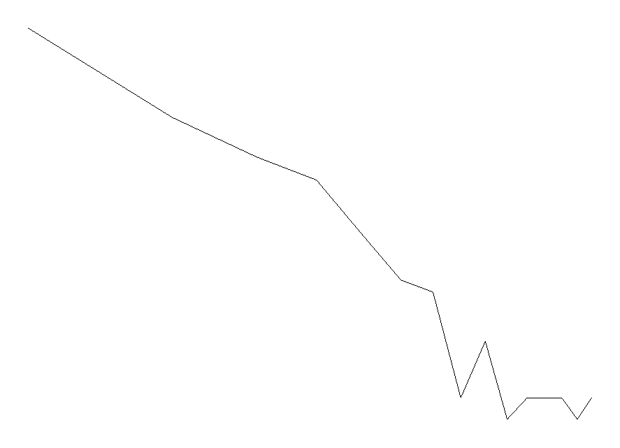
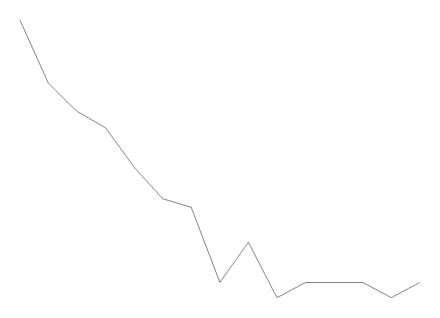
and we can see that the first 20 gaps decrease smoothly. To visually accept the Zipfian distribution as opposed to the exponential distribution we will produce two plots. (Notice that accepting a linear cost penalty function for deletions, is equivalent to accepting that the distribution of gaps is exponential.) The first one is a log-log plot, where a purely Zipfian distribution will show as a straight line.
DrawPlot( [ seq( [ln(i),ln(G[i])], i=1..15 )] ):

An exponential distribution would show as a straight line in a semi-log plot of the distribution. The semi-log plot is definitely curved, so we reject the exponential distribution in favour of a Zipfian one. Of course, more data would show the difference more markedly.
DrawPlot( [ seq( [i,ln(G[i])], i=1..15 )] ):

To show the agreement between the data and the Zipfian distribution we show the expected values and cumulatives for the first 20 gap lengths. We will use the value t=1.5 that was proposed in the paper and as it can be seen, fits the data very well.
k := sum(G[1..20]) / sum( 1/i^1.5, i=1..20 );
for i to 20 do
   printf( '%3d    %3d %6.1f    %3d %6.1f\n', i,
      G[i], k/i^1.5,
      sum(G[j],j=1..i), k * sum(1/j^1.5,j=1..i)) od;
k := 411.8521
  1    438  411.9    438  411.9
  2    142  145.6    580  557.5
  3     82   79.3    662  636.7
  4     54   51.5    716  688.2
  5     54   36.8    770  725.0
  6     20   28.0    790  753.1
  7     22   22.2    812  775.3
  8     18   18.2    830  793.5
  9     11   15.3    841  808.8
 10      9   13.0    850  821.8
 11      9   11.3    859  833.1
 12      8    9.9    867  843.0
 13      6    8.8    873  851.8
 14      7    7.9    880  859.6
 15      6    7.1    886  866.7
 16      3    6.4    889  873.2
 17      2    5.9    891  879.0
 18      0    5.4    891  884.4
 19      1    5.0    892  889.4
 20      2    4.6    894  894.0
© 2011 by Gaston Gonnet, Informatik, ETH Zurich
Last updated on Wed Oct 5 21:34:22 2011 by GhG
!!! This document is stored in the ETH Web archive and is no longer maintained !!!