Description of the algorithms and simulation results

We divide the algorithms in two groups. First the algorithms which produce a classification. Second the algorithms which take a classification and refine it (improve it).

1. Initial classification algorithms

   The initial classification algorithms compute a hyperplane that divides the space in the best possible way. There are several paradigms for computing this hyperplane.
   
   

   1. Least Squares.
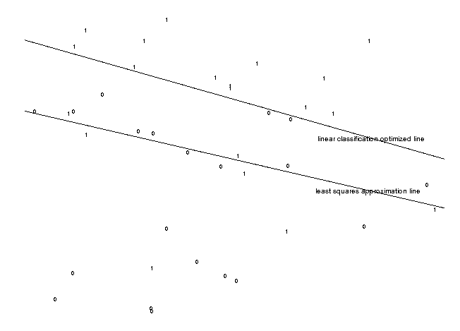
      These are algorithms which find a least squares approximation such that the positives are approximated to 1 and the negatives to 0. If the approximation is succesful, then the resulting linear form will be quite effective when compared to x₀=1/2. For the resulting approximation, the best cut point (x₀) is selected (it is not necessarily 1/2). In general, a least squares approximation looks like this
      
      
      In this case the least squares line is "pulled" down due to the some of the negatives which are relatively far from the main group. There is a much better division, found by linear classification, which sacrifices a pair of positives to correctly classify 9 negatives.
      There are two methods for doing this least squares approximation:
      
      
      1. BestBasis(k)
         A subset of size k of the independent variables is selected to do a least squares approximation. The subset is selected so that it gives the least error of the approximation. This is not an absolute minimum, just an approximation. For the simulations we have selected Best Basis of size 10. We could have used 4 or 5 depending on the problem which would give very good results. This would be sort of cheating, but on the other hand it is possible to do BestBasis for each of the sizes from 1 to n.
      
      
      
      2. Svd(val) or Svd(First(k)) (Singular value decomposition)
         A least squares approximation using svd is computed. The singular values used depend on the mode: for the first mode, all singular values >= val are used; for the second mode, the largest k singular values are used. The mode Svd(1.e-8) usually works very well, it discards linear dependencies of the independent variables and considers all the rest of the information.
      
      Tha main problem with the least squares methods is that they fail with two types of points: a point which is correctly classified but whose value is way too large (any change is useless) or a point which is incorrectly classified and whose value is hopelessly far from becoming correct. In these two cases, least squares methods will try to modify the answer to accomodate for this, which is not useful.
   
   
   
   2. Centre of Mass
      This method is very simple, it computes the centre of mass (centre of gravity, midpoint) of the positives and of the negatives and uses the direction between these two as perpendicular to the dividing hyperplane.
   
   
   
   3. Variance discrimination method
      This method computes, for each dimension, the distribution of the positives and the negatives. It then assumes that these distributions are normal and computes the probability p of making a false decision based on the best possible cut point. The coefficient for that dimension is computed as -ln(2p)
   
   
   
   4. Fisher linear discriminant
      Fisher's linear discriminant is a method coming from statistics which has a very intuitive description. It computes a vector x, such that the average Ax computed over the positives and the average Ax computed over the negatives are as far apart as possible relative to their variance.
   
   
   
   5. Logistic function
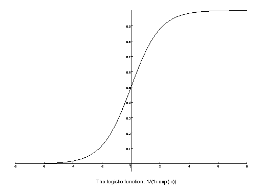
      The logistic function is logistic(x) = 1/(1+exp(-x)).
      
      
      
      It has the property of concentrating distant values into 0..1 while preserving linearity around 0. We apply the logistic function on A_ix and approximate it by least squares to 0 for the negatives and to 1 for the positives. In simpler terms, the function minimized is the sum of (1-logistic(Aix))^2 for the positives and logistic(Aix)^2 for the negatives. This is a non-linear least squares problem and it is resolved by iteration. In this case we use steepest descent (SD) starting from x=0 and using small steps so that we can guarantee that we are decreasing in the direction of the gradient. The problem has a minimum at an infinite norm, so the SD procedure is stopped after 200 steps.
   
   
   
   6. Cross entropy method
      This is very similar to the logistic method, except that the function to minimize is the cross entropy (when the logistic is viewed as a probability). In simpler terms, the function minimized is the sum of -ln(logistic(Aix)) for the positives and -ln(1-logistic(Aix)) for the negatives. This function is minimized in terms of x using steepest descent as for the logistic.
   
   
   
   7. Best(k)
      This is not a basic method, actually is an intertwined combination of several methods run with different starting points, chosing the best result at the end. The parameter k determines how long the algorithm will run, the longer, the better the results should be. The details of Best are not described here, as it changes from time to time as we find better strategies.
   
   
   



2. Refinement algorithms

   The refinement algorithms take an initial classification and change it if it can be improved. Otherwise it is left as is. For the refinements we always try to minimize the weighted number of misclassifications (errors). We have 4 basic forms of refinement. Two of them admit an additional parameter in the form of a distribution.
   
   

   1. Midpoint
      This refinement takes each dimension (independent variable) at a time and explores the interval where the minimum happens, leaving the value at the midpoint of the interval. If a lower number of errors is found, the coordinate is set to this new interval. If 0 is included in the interval, then that variable is set to 0.
   
   
   
   2. Swath or Swath(distribution)
      This refinement computes a least squares approximation of the points that lie close to the decision hyperplane. This is called a swath of the hyperplane, or a hyperswath. The number of points considered is randomly chosen between n and 3n. Once that the number of points is decided, the closest points to the decision hyperplane are selected. Each point is weighted according to the parameter distribution. (Currently the "triangular", "uniform" and "normal" distributions are supported). A least squares approximation is done approximating the positives to 1 and the negatives to -1. The resulting direction is used to attempt to improve the classification. This method of refinement is the most successful in practice as can be seen in the simulation results.
   
   
   
   3. Random
      This refinement uses a random direction and checks whether in this random direction we are at a minimum. If not it moves to the minimum. This refinement is not very effective.
   
   
   
   4. Progressive or Progressive(distribution)
      This refinement does a progressive reduction of the hyperswath (like in Swath) from the full size of the set down to n. This is done so that each hyperswatch size is roughly 90% of the previous size. The reduction size is randomly chosen. In some cases this refinement does better than all the other methods although it is quite time consuming.
   
   
   
3. Simulation results

   The simulation results use a matrix of independent variables with random values U(0,1). This matrix has 1000 rows and 25 columns (like 1000 data points with 25 values each; m=1000, n=25). The difference between the simulations is given by the way that the positives/negatives are determined.

   The score column shows the average score which is the weighted falses (weighted so that the all the positives weigh the same as all the negatives). Lower scores are better.

   The time is in seconds.

   The quality column is only available for the non-random simulations. It measures the alignment of the computed hyperplane with the one used for the construction of the positives/negatives (which is known to us). The measure is the normalized internal product, so a value of 1 is a perfect result, a value of 0 is a perfectly orthogonal result. It should be noticed that almost independently of the model, method, and simulation, the lower the score, the better the quality.

   Values in green indicate the best value for the column.

   Random In this simulation the positives are decided randomly, so any classification is a random result. It serves as the null hypothesis of classification.

   Deterministic This simulation uses a linear combination of the entries to determine positives. In particular, if A[i,3]-3*A[i,4]+7*A[i,5] > 1/2 is true then the row is considered a positive.

   Deterministic+Noise This simulation uses a linear combination of the entries plus some random noise to determine positives. In particular, if A[i,3]-3*A[i,4]+7*A[i,5]+Rand() > 1/2 is true then the row is considered a positive.

   Deterministic-full direction + Noise This simulation uses a linear combination of the entries plus some random noise to determine positives. In particular, if A[i]*Direction+Rand()/4 > 1/2 is true then the row is considered a positive. Direction is a random direction in n dimensions.
   
   

Some of the conclusions are obvious.

The construction methods are uniformly mediocre to poor compared against the Best method. Notice that the Best method is much better, but it also requires more time. One exception is Svd(First(10)) which is much worse than the others. Using just a few singular values appears to be a poor choice.

As an initial method, we choose Svd(1e-8), as it gives results as good as the best and it takes only a fraction of the time.

Any initial method is much worse than Svd(1e-8) plus one iteration of refinement. In particular Swath appears to be the most effective refinement. (Progressive is better, but it takes much longer.)

The weight distributions for Swath and Progressive are roughly equivalent with a minor edge in favour of normal.

The Random refinements are, as expected, the weakest refinements.

Index of bio-recipes

Last updated on Sat Feb 8 20:28:51 2003 by GhG