This bio-recipe shows an algorithm that resolves the haplotypes from genotype information. The input is a matrix that contains n genotype sequences and gives back a matrix containing 2n haplotype sequences. The idea and the algorithm base on a paper of Richard Karp et al. (R.M.Karp, E.Eskin, E.Halperin: Large Scale Reconstruction of Haplotypes from Genotype Data).
The genetic basis of complex disease have its seeds often in the modeling of human variation. Most of this variation can be characterized by single nucleotide polymorphisms (SNPs) which are mutations at a single nucleotide position that occured once in human history and were passed on through heredity. To characterize an individual's variation, we must determine an individual's haplotype or which nucleotide base occurs at each position of these common SNPs for each chromosome.
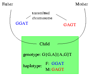
With the current technology it is possible to get the genotype of an individual and to determine the positions of the SNPs. The genotype gives the bases at each SNP for both copies of the chromosome but loses the information of the origin. We will explain it on the following example:
Let's say that the child is diseased. To characterize its disease we have to look at its genetic background. Therefore we go to the lab where we can get the genotype of the child. The genotype shows us that (in this example) on the first position only a T occurs ; therefore we know that both the transmitted chromosome of the father and the transmitted chromosome of the mother have a T on their first position. On the second position the gentoype shows that the child got a G and an A occur but it does not store the information as which base comes from which chromosome. On the third position we have again two bases and it is impossible to say which base from the second position lies with which base on the third position on one of the chromosomes.
The haplotype of the child shows the two transmitted chromosomes seperatly; this presentation allows us to determine which bases lie together on which chromosome.
The earliest method to resolve the haplotypes assumes that you have the genotype data from a whole trio (mother, father and child). By applying the known rules of inheritance it is obvious that we can get the haplotypes in almost all cases. But to collect all this data is very difficult and sometimes impossible because the genotype data from one of this trio could not exist any more. The present method does not need to collect any data from related individuals; it resolves the haplotypes from genotype sequences without any additional information about the relations between them. To be able to do that (and to br able to do that even in a reasonable time) some assumptions about the data are made.
The two chromosomes a child gets are not exactly the same than the chromomosomes of its parents. During reproduction there are exchanges of segments of DNA on the two chromosomes of the father as well as of the mother what leads to a novel combination of genetic material in the offspring.
These exchanges of segments of DNA are called recombinations. These recombinations do not take place randomly over the genome; there are locations where exchanges of DNA takes place most frequently. We illustrate it on the following picture:
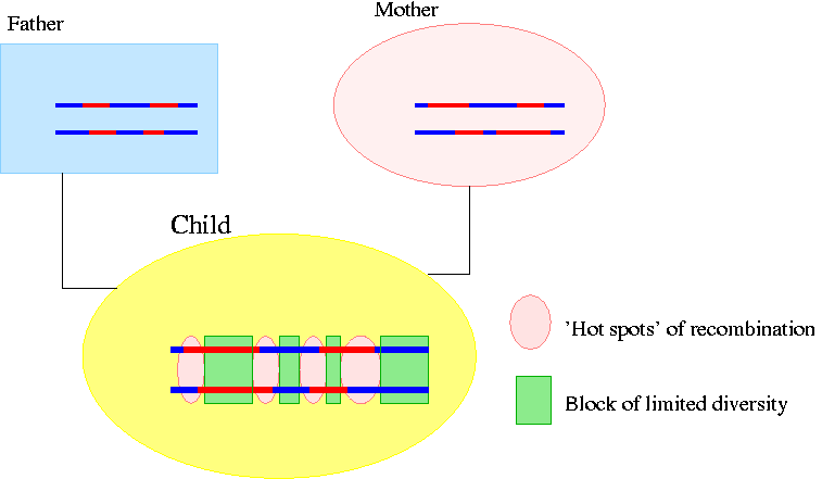
The changes of color show where recombination happened (The recombinations on the chromosomes of the father and the mother happened on the DNA of their ancestors). You can see that on the DNA of the child there are four regions ('hot spots') where recombination took place most frequently that divide the chromosomes into blocks. We make the next assumption about these blocks:
In the blocks between the 'hot spots' they observed that no recombination takes place. Therefore these blocks stay conserved through inheritance.
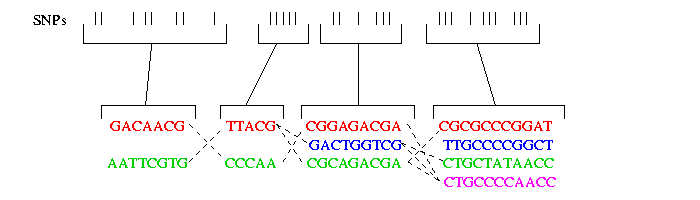
On the following picture you can see four such blocks containig several SNPs. As you can see not more then 4 haplotypes occur in one block. In each block in general containing n SNPs, typically not more then four haplotypes account for the majority of the haplotypes of the population.
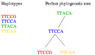
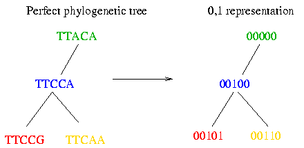
As you can see the haplotypes within a block did not evolve very much. Therefore it is possible to fit them to a perfect phylogenetic tree. The perfect phylogenetic tree implies that a mutation on a certain site happens only once in human history. This constraint forbids recurrent or back mutations. In the following picture you see four haplotypes from a block and how you can fit them to a perfect phylogenetic tree:
Of course the perfect phylogenetic tree model is a very strict model and not all data fit the perfect phylogenetic tree. Therefore some heuristics are introduced that make the algorithm work in practice. These heuristics will be explained later in this bio-recipe.
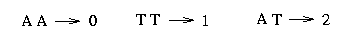
Since there are only two observed bases for the vast majority of SNPs, we can denote these nucleotides by 0 and 1. (Although this assumption seems artificial, it is the case in most polymorphic sites.) The following picture shows you how to transform the tree built in the 3. Assumption into the 0 and 1 representation:
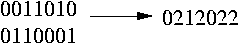
The genotype is represented with the elements {0,1,2}. There is a 0 or a 1 at the polymorphic site of the genotype if the two chromosomes contain the same base at this site and a 2 if the bases on this site differ.
In the following picture you can see two transformed haplotypes and how to transform them into the genotype:
We have a bunch of genotype sequences and we split these sequences into blocks. Th haplotypes are resolved for each block seperately. Since we are interested in the inheritance pattern of the mutations (which are probably triggers for diseases) only the SNPs are selected to do the procedure of finding the haplotypes. The SNPs are converted into the 0,1 and 2 representation as mentioned above. All these {0,1,2} sequences (for each sequence the transformed SNPs of the first block) are stored in a matrix. We call it the genotype matrix. The elements of this matrix are 0, 1 and 2. The goal now is to find a haplotype matrix that:
1. contains for every sequence in the genotype matrix two haplotype sequences that are compatible* with the genotype sequence.
2. fits a perfect phylogenetic tree.
* compatible: two sequences a and b are compatible with a sequence c if for every site i the following holds:
1. if a(i) = b(i) then a(i) = b(i) = c(i)
2. if a(i) <> b(i) then c(i) = 2
For example:
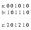
The sequences a and b are compatible with the sequence c.
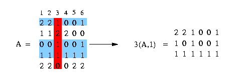
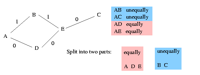
We use the notation c(A,x) to mention the set of rows of matrix A containing the value x at column c. In the following example we have a matrix A and we want to get all rows that contain a 1 at column 3:
We say that column c1 and column c2 induce (x,y) if there are rows that fulfill the condition, that they contain in column c1 either a x and in column c2 a y or in column c1 a x and in column c2 a 2 or in column c1 a 2 and in column c2 a y. Look at the following example: We have a matrix A (see in the picture below) and want to know if column 3 and column 4 induce (1,0). We can easily see that column 3 and column 4 contain pairs that fulfill the condition and therefore column 3 and column 4 induce (1,0). The columns 1 and 2 - to make an other example - don't induce (1,0) because there is no pair that fulfills the condition.
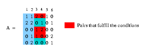
(If two columns induce all the for possible states (0,0),(0,1),(1,0),(1,1) it is not possible to build a phylogeny tree and therefore the number of pairs that are induced by two certain columns has to be smaller than four.)
We have stored all the data in the file data.txt in the directory Haplotypes. The data consist of 387 sequences, these are the 129 trios (father, mother and child) we mentioned in the chapter 'Data'. Each sequence shows the two bases (that lie on the two chromosomes) for all 103 SNPs. To run the algorithm we pick the genotypes of the children; the sequences of the parents are necessary to verify the result. To illustrate how such a seuquence looks like we show one sequence of a child:
ReadProgram( 'Haplotypes/data.txt');
print(AllTrios[2]);
[PED054, 412, 430, 431, 2, 2, 1, 3, 1, 3, 4, 1, 4, 2, 2, 1, 3, 1, 4, 2, 3, 2, 3,
3, 2, 4, 2, 4, 2, 1, 1, 2, 1, 3, 2, 2, 2, 2, 3, 3, 0, 0, 1, 1, 3, 3, 1, 1, 2, 2,
3, 3, 1, 1, 2, 2, 4, 3, 3, 2, 2, 3, 4, 2, 1, 2, 4, 2, 1, 3, 1, 3, 2, 1, 2, 4, 3,
2, 2, 2, 3, 1, 2, 2, 4, 2, 2, 2, 4, 4, 3, 3, 1, 1, 2, 4, 4, 2, 2, 2, 2, 2, 2, 4,
1, 3, 4, 2, 2, 4, 2, 4, 1, 1, 4, 2, 2, 3, 1, 3, 4, 4, 3, 3, 3, 2, 4, 1, 2, 3, 3,
4, 1, 3, 1, 3, 4, 2, 3, 1, 2, 2, 3, 3, 4, 4, 1, 1, 2, 4, 1, 4, 3, 4, 4, 2, 1, 1,
2, 2, 4, 2, 3, 3, 4, 4, 4, 4, 4, 4, 3, 1, 1, 3, 0, 0, 3, 1, 2, 2, 1, 3, 3, 1, 4,
2, 0, 0, 4, 3, 3, 4, 4, 4, 3, 2, 2, 4, 3, 3, 3, 1, 2, 4, 3, 1, 3, 4, 2, 1, 3, 3]
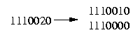
The sequence starts from the 7th position. Every two consecutive bases belong together and express the bases on the two chromosomes, the one from the father and the one from the mother. A 1 stands for 'A', a 2 for a 'C', a 3 for a 'G' and a 4 for a 'T'. To get the genotype sequences we convert these sequences in the following way: Since we assume that at each SNP at most two different bases appear we assign a 2 to a certain site if the bases on the two chromosomes differ and a 0 (or 1) otherwise. For example at the first site we assume to have either an 'A' or a 'T', therefore we make the following assignment:
As mentioned above the haplotypes are split into 11 blocks. The algorithm is performed for every block. We pick the second block of the genotypes and show the procedure on this example. The genotypes of this block contain five SNPs and the assignment of the bases looks as follows:
ReadProgram( 'Haplotypes/2ndblock.txt');
The second block is now assigned to A. To see how it looks like, we print the first five sequences:
print(A[1..5]);
[
 [2, 2, 2, 2, 2]
 [2, 2, 2, 2, 2]
 [1, 1, 0, 1, 1]
 [1, 1, 0, 1, 2]
 [1, 1, U, 1, 1]
]
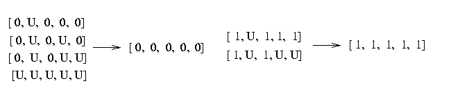
As already mentioned, the 1's in the genotypes resolve to 1's in the haplotypes and the 0's to 0's. A 'U' stands for a missing site and those sites are ignored in the following computations. The difficulty is to resolve each 2 to either a (0,1) or a (1,0) in a consistent way, so that the resulting haplotypes correspond to the perfect phylogenetic tree model.
To simplify the following procedures, we create a list that contains all the columns that we are considering.
ColumnList:= {1,2,3,4,5}:
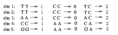
We convert now the matrix in the following way: Using our freedom to decide which of the nucleotides at a polymorphic site shall be designated 1, we may assume without loss of generality that the root of the tree is the all zeros vector. This implicates that any two columns induce (0,0). We obtain this by changing the matrix in the following way: By complementing certain columns (i.e., replacing 0 by 1 and 1 by 0 throughout the column) one can ensure that in each column c, either every row contains a 2 or a 0 appears in the first row not containing a 2. We illustrate it in the following picture:
With this condition we can assure that any two columns induce (0,0).
Three columns has to be changed that the above condition is fulfilled. Now it is easy to see (look at the resulting matrix) that unless there are two identical columns of 2's, any two sites induce (0,0). We do this convertion in the procedure ConvertMatrix().
ConvertMatrix := proc( a:list(list) )
A := transpose(a):
Swap := CreateArray(1..length(A));
for i to length(A) do
    for j to length(A[1]) do
	if A[i,j] = 0 then break;
	elif A[i,j] = 2  or A[i,j] = 'U' then next;
	else
	    Swap[i] := 1;
	    for j to length(A[1]) do
	        if A[i,j] <> 'U' and A[i,j] <> 2 then
		   A[i,j] := 1 - A[i,j];
		   fi;
		od;
	    fi;
	od;
    od;
Res := [transpose(A),Swap];
return(Res);
end:
Res := ConvertMatrix(A):
A := Res[1]:
The first five sequences of the converted matrix are shown below:
print(A[1..5]);
[
 [2, 2, 2, 2, 2]
 [2, 2, 2, 2, 2]
 [0, 0, 0, 0, 0]
 [0, 0, 0, 0, 2]
 [0, 0, U, 0, 0]
]
The Array Swap stores the columns that have been converted:
Swap := Res[2];
Swap := [1, 1, 0, 1, 1]
We note the columns that we changed in the array 'Swap' in order to change these columns back at the end of the computation.
Now we remove the columns that appear twice and contain at least one 1. All 2's in these equal columns that contain a 1 have to be resolved equally; if they are resolved unequally (what would mean (2,2) --> (0,1) and (1,0)), two columns would contain all four pairs (0,0) (according to our condition above), (0,1), (1,0) and (1,1). That would make a construction of the phylogenetic tree impossible. We illustrate it in the following picture:
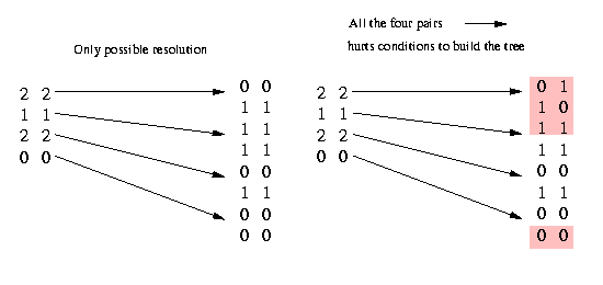
As you can see, the only possible way - if the identical columns contain at least one 1 - not to have all the four pairs is by resolving all the (2,2) pairs equally. (If we have no 1 in the two equal columns we can resolve the (2,2) pairs either equally or unequally, therefore we can not remove identical columns that do not contain a 1.)
Removing columns is done in the following procedure RemoveIdColumns():
RemoveIdColumns := proc( Co:set, a:list(list) )
CoLi := Co;
A := transpose(a):
RemoveList := CreateArray(1..length(A));
for i to length(A)-1 do
    for j from i+1 to length(A) do
	p := 1;
	if member(1,A[i]) then
	    while p <= length(a) and (A[i,p] = A[j,p] or A[i,p] ='U' or A[j,p] = 'U')  do
	        p := p+1;
	        od;
	    fi;
	if p = length(a)+1 then
	    RemoveList[j] := i;
	    CoLi := CoLi minus {j};
	    fi;
	od;
    od;
Result := [CoLi,RemoveList];
return(Result);
end:
Result := RemoveIdColumns(ColumnList,A):
RemoveList := Result[2];
RemoveList := [0, 0, 1, 0, 0]
In this case, column 3 is equal to column 1 and has been removed.
ColumnList := Result[1];
ColumnList := {1,2,4,5}
With the matrix A we can start to compute the tree.
We define the following relations between two columns:
Strong Domination: c is ancestor of c' -> (c,c') induce {(0,0),(1,0),(1,1)}
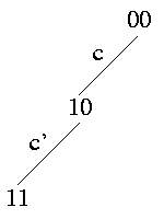
All rows in the matrix that have a 1 at site c' also have a 1 at site c. The path in the tree from the root to the edge c' leads necessarily over edge c.
Siblings: c and c' are siblings -> (c,c') induce {(0,0),(0,1),(1,0)}

All rows in the matrix that have a 1 at site c can not have a 1 at site c'. There is no path in the tree that encounters both edges c and c'.
Weak Domination: c weakly dominates c' -> (c,c') induce {(0,0),(1,0)} or {(0,0)}
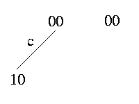
The weak domination expresses that there is no row in the matrix that contain a 1 in column c'. Therefore the branch that is assigned to c' does not exist in the tree. This is the only ambiguous case where we cannot definitely determine how to resolve it.
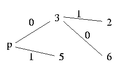
For each pair c and c' exactly one of the above relations holds. Therefore we define a pivot column as follows: Since strong domination and weak domination both induce a linear order on the columns, the pivot column is a maximal element with respect to both orders; in other words the pivot column has no ancestor. Look at the following example:
As you can see, the 'highest' columns are either column 2 or column 4 and both of them can be choosen as the pivot column.
We want to know the relation between the columns. The relation is determined by the set of different pairs that induce these two columns. So we define the Inductionset that holds all the pairs between two coloumns that induce the two columns (if you forgot what induce means, read here).
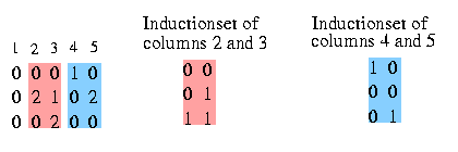
You see the Inductionset of pairs that induce column 2 and 3. The pairs in the Inductionset for two specific columns will occur in the resulting haplotypes in these columns. This set reveals also the relation between the two columns, in this case we see that column 3 strongly dominates column 2. The same with column 4 and 5: the Inductionset for them determines that column 4 and 5 are siblings.
The Inductionset is computed in the following procedure:
GiveInductionSet := proc( c1:integer, c2:integer, Co:set, a:list(list) )
IndSet := {};
A := transpose(a);
SetOfPairs := {op(transpose([A[Co[c1]],A[Co[c2]]]))};
for z in SetOfPairs do
    if z = [2,2] or member('U',z) then else
        if member(2,z) then
	    if z[1] = 2 then
		IndSet := append(IndSet,[0,z[2]],[1,z[2]]);
	    else
		IndSet := append(IndSet,[z[1],0],[z[1],1]);
	    	fi;
    	else
		IndSet := append(IndSet,z);
		fi;
	fi;
od;
return(IndSet);
end:
For example for column 1 and column 2 we get the following Inductionset:
GiveInductionSet(1,2,ColumnList,A);
{[0, 0],[0, 1],[1, 1]}
It can occur that the set contains the four pairs, (0,0), (0,1), (1,0) and (1,1) as for column 2 and column 4.
GiveInductionSet(2,4,ColumnList,A);
{[0, 0],[0, 1],[1, 0],[1, 1]}
In this case the set contains all four pairs and therefore it is impossible to build the phylogenetic tree. Either one column strongly dominates the other or they are siblings, but they can not be both. To be sure to get a solution anyhow we have to weaken the constraint of the phylogenetic tree model. Therefore we define two heuristics that guarantee to build a tree in all cases:
We define a threshold which is a under limit of the amount of occurrences of a certain pair. For example if we set the threshold to the value 3, all the pairs that occur less than 3 times are removed.
GiveInductionSetWithThreshold := proc( c1:integer, c2:integer, k, Co:set, a:list(list) )
Count := CreateArray(1..2,1..2);
#In the Count matrix we store the counts for [0,1] at position [1,2],
#for [1,0] at position [2,1] and for [1,1] at position [2,2]
IndSet := {};
for i to length(a) do
    FirstEl := a[i][Co[c1]]; SecondEl := a[i][Co[c2]];
    if not(([FirstEl,SecondEl] = [2,2]) or (member('U',[FirstEl,SecondEl]))) then
    	if member(2,[FirstEl,SecondEl]) then
	    if FirstEl = 2 then
		IndSet := append(IndSet,[0,SecondEl],[1,SecondEl]);
		Count[1,SecondEl+1] := Count[1,SecondEl+1] + 1;Count[2,SecondEl+1] := Count[2,SecondEl+1] + 1;
	    else
		IndSet := append(IndSet,[FirstEl,0],[FirstEl,1]);
		Count[FirstEl+1,1] := Count[FirstEl+1,1] + 1;Count[FirstEl+1,2] := Count[FirstEl+1,2] + 1;
		fi;
	else
	    IndSet := append(IndSet,[FirstEl,SecondEl]);
	    Count[FirstEl+1,SecondEl+1] := Count[FirstEl+1,SecondEl+1] + 1;
	    fi;
	fi;
    od;
if Count[1,2] <= k then
    IndSet := IndSet minus {[0,1]};
elif Count[2,1] <= k then
    IndSet := IndSet minus {[1,0]};
elif Count[2,2] <= k then
    IndSet := IndSet minus {[1,1]};
    fi;
if length(IndSet) <= 3 then
    return(IndSet);
else
    RemovePair(IndSet,Count);
    fi;
end:
Let's check if the thereshold of 1 was enough high to shrink the set to less then four pairs:
IndSet := GiveInductionSetWithThreshold(2,4,1,ColumnList,A);
IndSet := {[0, 0],[1, 0],[1, 1]}
The pair [0,1] occurs only one time, so it is skipped from the Inductionset. In the case that the first heuristic is not strong enough (i.e. there would have been two pairs of [0,1] in the Inductionset ) we have to define a second heuristic.
The second heuristic just counts the occurrences of every pair and removes the one that occurs least. With this heuristic we can guarantee that in every Inductionset there are at most three pairs.
RemovePair := proc( IndSet:set, Count:list )
    if Count[1,2] < Count[2,1] and Count[1,2] < Count[2,2] then
	IndSet := IndSet minus {[0,1]};
    elif Count[2,1] < Count[1,2] and Count[2,1] < Count[2,2] then
	IndSet := IndSet minus {[1,0]};
    else IndSet := IndSet minus {[1,1]};
    fi;
return(IndSet);
end:
With these heuristics we can guarantee that every two columns induces at most three pairs and therefore the perfect phylogenetic tree is realizable. After making these preparations and checking that each two columns induce (0,0) (what is a necessary condition, as discussed above) we can start to compute the relations between every two columns.
We define a matrix Relations where we store the information about the relation between any columns in the following way: A 1 is assigned to the position [i,j] if column i is ancestor of column j (and automatically a -1 to the positon [j,i]). When column i and j are siblings we assign a 2 to the position [i,j] and to the position [j,i]. When column i weakly dominates column j then we assign a 3 to Relations[i,j] and a -3 to Relations[j,i].
ComputeRelations := proc( Co:set, a:list(list) )
Relations := CreateArray(1..length(Co),1..length(Co));
for i to length(Co)-1 do
    for j from i+1 to length(Co) do
        InductionSet := GiveInductionSet(i,j,Co,a);
	if  ((length(InductionSet)) >= 4) then
	    InductionSet := GiveInductionSetWithThreshold(i,j,1,Co,a);
	    fi;
	if member([0,0],InductionSet) and ((length(InductionSet)) <= 3) then
            if InductionSet = {[0,0],[1,0],[1,1]} then
		Relations[i,j] := 1;Relations[j,i] := -1;
	    elif InductionSet = {[0,0],[0,1],[1,1]} then
		Relations[j,i] := 1;Relations[i,j] := -1;
	    elif InductionSet = {[0,0],[0,1],[1,0]} then
	        Relations[i,j] := 2;Relations[j,i] := 2;
	    elif InductionSet = {[0,0],[0,1]} then
	        Relations[j,i] := 3; Relations[i,j] := -3;
	    elif InductionSet ={[0,0],[1,0]} or InductionSet ={[0,0]} then
	        Relations[i,j] := 3; Relations[j,i] := -3;
	    else
	        printf('sites %d and %d fulfill none of the expected relations\n',i,j);
	        fi;
	else
	    printf('Condition not fulfilled for columns %d and %d,Inductionset = %a\n',i,j,InductionSet);
	    Relations[i,j] := 4;Relations[j,i] := 4;
	    fi;
	od;
    od;
return(Relations);
end:
Relations := ComputeRelations(ColumnList,A);
Relations := [[0, -1, 1, -1], [1, 0, 1, 1], [-1, -1, 0, -1], [1, -1, 1, 0]]
The Relations matrix stores all the information we need to compute the pivot column, that means the column that is the highest in the tree.
We get the pivot column by going through the matrix and looking for the maximal element:
FindPivot := proc( Co:set, rel:list(list) )
pivot := 1;
for i to length(rel) do
    if rel[pivot,i] = -1 or rel[pivot,i] = -3 then
	pivot := i;
	fi;
    od;
return(pivot);
end:
pivot := FindPivot(ColumnList,Relations);
pivot := 2
Column 2 is the maximal element according to the linear order of the strong and the weak domination; therefore column 2 is our pivot. This is the column that is resolved first.
The resolution of a row that contains at most one 2 is obvious:
The difficult case we have to deal with is if the row contains more then one 2:
To handle this case we have to determine whether we resolve a pair in a certain row (2,2) either equally or unequally.
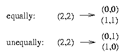
It is impossible to resolve two columns both equally and unequally because that would mean that the resulting matrix contains in two columns the four pairs (0,0), (1,0), (0,1) and (1,1). Therefore our task is to decide if we resolve two columns equally or unequally.
The algorithm now proceeds to resolve the rows that contain a 2 in the pivot column p. Every column that is a child of p must be resolved equally with p. Every column that is a sibling of p must be resolved unequally with p. It remains to decide which columns that are weakly dominated by p are to be resolved equally with p and which are to be resolved unequally with p.
To make this determination the algorithm constructs a graph Gp whose vertex set is the set of sites. There is an edge labeled 0 between p and each column that is a child of p. There is an edge labeled 1 between p and its siblings. If column c and column d are sites different from p then there is an edge between c and d labeled 0 if there is a row that contains a 2 in all three columns and column c and column d induce (1,1); they have to be resolved equally. If column c and column d are sites different from p then there is an edge between c and d labeled 1 if there is a row that contains a 2 in all three columns and column c and column d are siblings; they have to be resolved unequally.
ConstructGraph := proc( pivot, rel:list(list), Co:set, a:list(list))
MyGraph := Graph({},{seq(i,i=1..length(Co))});
A := transpose(a);
for j to length(rel) do
    if member([2,2],transpose([A[pivot],A[Co[j]]])) then
	if rel[pivot,j] = 1 then
	    MyGraph[Edges] := append(MyGraph[Edges],Edge(0,pivot,j));
	elif rel[pivot,j] = 2 then
	    MyGraph[Edges] := append(MyGraph[Edges],Edge(1,pivot,j));
	    fi;
	fi;
    od;
for i to length(rel)-1 do
    for j from i+1 to length(rel) do if i <> j and i <> pivot and j <> pivot then
    	if member([2,2,2],transpose([A[pivot],A[Co[i]],A[Co[j]]])) then
	    if rel[i,j] = 1 then
		MyGraph[Edges] := append(MyGraph[Edges],Edge(0,i,j));
	    elif rel[i,j] = 2 then
		MyGraph[Edges] := append(MyGraph[Edges],Edge(1,i,j));
		fi;
	    fi;
	fi;od;
    od;
return(MyGraph);
end:
We get the following graph:
MyGraph := ConstructGraph(pivot,Relations,ColumnList,A);
MyGraph := Graph(Edges(Edge(0,2,1),Edge(0,2,3),Edge(0,2,4),Edge(0,1,3)),Nodes(1,
2,3,4))
The graph in the following picture does not correspond to the above graph since the computed graph does not contain all cases. Therefore - just to illustrate all different resolutions - it is easier that we construct a graph by ourselves that contains all possible cases.
Let's say that the graph has six nodes and the pivot is column 4:
As we can read out from the graph, column 5 is a sibling of p and has to be resolved unequally, column 3 is a child and therefore has to be resolved equally. Since column 3 is a child of p and column 2 a sibling of column 3, column 2 has also to be sibling of column p and hence has to be resolved unequally with p. And in contrast column 6 is a child of 3 and 3 is child of p, therefore column 6 has also to be a child of p; so we resolve 6 equally with p.
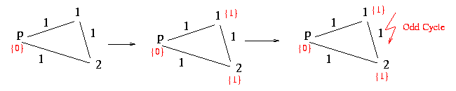
If there exists an odd cycle in the graph - what means a cycle that contains an odd number of edges labeled 1 - it is impossible to resolve the genotypes.
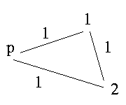
p is a sibling of 1, 1 a sibling of 2 and 2 sibling of p. If we have this case it is impossible to resolve the genotypes.
The following procedure checks if there is an odd cycle or not. It starts at the first node and marks it with a 0. The algorithm now proceeds by setting a marker to all adjacent nodes in the following way: If the interjacent edge between two nodes is labeled with a 0 the algorithm marks the new node with same marker as at the adjacent node. If the edge is labeled with a 1 the marker skips from a 0 to a 1 or from a 1 to a 0. If there is a conflict between two nodes that are linked and already marked the algorithm returns false.
NoOddCycle := proc( g:structure )
state := CreateArray(1..length(g[Nodes]),-1);
for i to length(state) do
    if state[i] = -1 then
	state[i] := 0;
	Q := [i];
	while length(Q) <> 0 do
	    u := Q[1];
	    if length(Q) = 1 then
		Q := [];
	    else
		Q := Q[2..length(Q)];
	        fi;
	    for v in (g[Adjacencies][u]) do
		if state[v] = -1 then
		    state[v] := mod(state[u]+g[Labels][u,v],2);
		    Q := append(Q,v);
		elif mod(state[u]+g[Labels][u,v],2) <> state[v] then
		    return(false);
		    fi;
		od;
	    od;
	fi;
    od;
return(true);
end:
Let's check if our graph has an odd cyle:
if NoOddCycle(MyGraph) then print('No odd cyle'); else print('Odd cycle in graph'); fi;
No odd cyle
Assume that we have a odd cycle in the graph. The graph would not be resolvable and we would not get a result. But since we want to have a result in the end we have to weaken the assumptions by defining a third heuristic.
The third heuristic assigns a notion of strength to each edge in the graph. The strength of an edge between c and d different from pivot is the number of rows that have a 2 at site c, site d and site pivot. If the graph contains an odd-weight cycle, we repeatedly remove the weakest edge until no cycle exists.
SolveOddCycle := proc( graph:structure, a:list(list), pivot,CoLi:set )
g := graph;
while not(NoOddCycle(g)) do
    count := CreateArray(1..length(graph[Nodes]),1..length(graph[Nodes]));
    for i in g[Edges] do
	if not(member(pivot,[i[2..3]])) then
	    for j to length(a) do
		if a[j][CoLi[pivot]] = 2 and a[j][CoLi[i[2]]] = 2 and a[j][CoLi[i[3]]] = 2 then
		    count[i[2],i[3]] := count[i[2],i[3]] + 1;
		    fi;
		od;
	    fi;
	od;
    min := 99999;
    for i to length(count)-1 do
	for j from i + 1 to length(count) do
	    if count[i,j] < min and count[i,j] > 0 then
		min := count[i,j];
		mark := [i,j];
		fi;
	    od;
	od;
    for i in g[Edges] do
	if ([i[2..3]] = mark) or ([i[3].','.i[2]] = mark) then
	    g := InduceGraph(g,Edges(i));
	    fi;
	od;
    od;
return(g);
end:
In our case the graph does not contain an odd cycle, therefore no edge has to be removed.
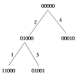
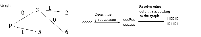
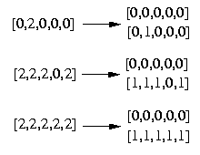
After computing the graph we can start to resolve the haplotypes. We show in an example how the algorithm works: Let's assume that we have a row that looks like 122222. We choose arbitrarily a resolution for the pivot colum 4. Then we resolve the other columns according to the graph (as explained here).
The columns that are weakly dominated by the pivot column lie in a different component of the graph. It remains to determine how these columns shall be resolved. The vertex set of each such component partitions uniquely into two parts, such that any two vertices in the same part must be resolved equally and any two vertices in different parts must be resolved unequally. In the following example we assume that the shown graph is a component different to the main graph (that includes the pivot). The five vertices A, B, C, D and E can be split into two parts as shown in the picture:
The algorithm arbitrarily resolves the vertices in one of these parts equally with p and the vertices in the other part unequally with p. In the above picture for example the algorithm chooses randomly to resolve A, D and E equally with p. Therefore C and B has to be resolved unequally with p.
Let's resolve the first genotype of our data.
A[1];
[2, 2, 2, 2, 2]
We have already computed the pivot and the graph that belong to the data:
pivot;
2
MyGraph;
Graph(Edges(Edge(0,2,1),Edge(0,2,3),Edge(0,2,4),Edge(0,1,3)),Nodes(1,2,3,4))
These parameters suffices to compute the haplotypes according to the explanation above. We do this in the following procedure:
ResolveTwoHaplotypes := proc( pivot:integer, seqs, Co:set, g:structure )
hap1 := copy(seqs);hap2 := copy(seqs);
G := g;
PathList := ShortestPath(G,pivot);
TPathList := transpose(PathList);
for j to length(Co) do
    if j = pivot then
	    hap1[Co[j]] := 0; hap2[Co[j]] := 1;
    elif seqs[Co[j]] = 2 then
        index := SearchArray(j,TPathList[1]);
        if index <> 0 then
            distance := PathList[index,2];
	    if mod(distance,2) = 0 then
	        hap1[Co[j]] := 0; hap2[Co[j]] := 1;
	    else
	        hap1[Co[j]] := 1; hap2[Co[j]] := 0;
	        fi;
        else
    	    #Node j lies in a different component
            if member(j,G[Nodes]) then
	        PathList2 := ShortestPath(G,j);
	        VertSet := {seq(PathList2[p,1],p=1..length(PathList2))};
 	        G := InduceGraph(G,Nodes(op(VertSet)));
		if seqs[Co[j]] = 2 then
	        if length(PathList2) = 1 then
	       	    hap1[Co[j]] := 0; hap2[Co[j]] := 1;
	        else
		    for k to length(PathList2) do
		        distance := PathList2[k,2];
		        #the nodes are split into two parts, one is (randomly) resolved equally, the other unequally
		        if mod(distance,2) = 0 then
			    hap1[Co[PathList2[k,1]]] := 0; hap2[Co[PathList2[k,1]]] := 1;
		        else
			    hap1[Co[PathList2[k,1]]] := 1; hap2[Co[PathList2[k,1]]] := 0;
			    fi;
		        od;
		    fi;fi;
	        fi;
            fi;
	fi;
    od;
Haplotypes := [hap1,hap2];
return(Haplotypes);
end:
Let's look how the first two haplotypes look like:
Haplotypes := ResolveTwoHaplotypes(pivot,[2,2,2,2,2],ColumnList,MyGraph);
Haplotypes := [[0, 0, 2, 0, 0], [1, 1, 2, 1, 1]]
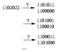
So these two Haplotypes are resolved from the genotype [2,2,2,2,2]. Don't care about the 2 in the third column, since we determined in the beginning that the third column will be ignored. We will replace the third column in the end with the first one. (So in this case the two haplotypes will look like [0,0,0,0,0] and [1,1,1,1,1]) We go forward and resolve all the genotypes which contain a 2 in the pivot column.
ResolveHaplotypes := proc( pivot, Co:set, a:list(list), g:structure )
Haplotypes := [];
Genotypes := {};
A := a;
remark := [];
HaplTogether := [];
for i to length(A) do
    if A[i,Co[pivot]] = 2 then
    	#Resolve sequence i at site pivot if there is a 2
	Genotypes := append(Genotypes,A[i]);
	haps :=  ResolveTwoHaplotypes(pivot,A[i],Co,g);
	HaplTogether := append(HaplTogether,op(haps));
	remark := append(remark,i);
	fi;
    od;
if length(remark) <> 0 then
    for p from length(remark) to 1 by -1 do
	if remark[p] = 1 then A := A[2..length(A)];
	elif remark[p] = length(A) then A := a[1..length(A)-1];
	else A := append(A[1..remark[p]-1],op(A[remark[p]+1..length(A)]));
	fi;
	od;
    fi;
A := append(A,op(HaplTogether));
Result := [A,Genotypes, HaplTogether];
return(Result);
end:
Result := ResolveHaplotypes(pivot,ColumnList,A,MyGraph):
Let's look at the genotypes we resolved; they should all contain a 2 in the 2nd column, the pivot column:
Genotypes := Result[2];
Genotypes := {[0, 2, 0, 0, 0],[2, 2, 2, 0, 2],[2, 2, 2, 2, 2]}
The following haplotypes come out:
Haplotypes := {op(Result[3])};
Haplotypes := {[0, 0, 0, 0, 0],[0, 0, 2, 0, 0],[0, 1, 0, 0, 0],[1, 1, 2, 0, 1],[
1, 1, 2, 1, 1]}
Also here we have to replace the third column with the first one to get the end result. The following picture shows clearer which genotype was resolved to which haplotypes.
To find out which haplotypes are most frequently we have to resolve all genotypes.
Resolve := proc( a:list(list), CoLi:set )
ColumnList := CoLi;
Rows := [];
Genotypes := a;
AllHaplotypes := [];
#take away all rows that do not contain a 2
for i to length(Genotypes) do
    if not(member(2,Genotypes[i])) then
	row := copy(Genotypes[i]);
	Rows := append(Rows,row);
	fi;
    od;
while ColumnList <> {} do
    Haplotypes := [];
    rel := ComputeRelations(ColumnList,Genotypes);
    pivot := FindPivot(ColumnList,rel);
    GenotypesT := transpose(Genotypes):
    if member(2,GenotypesT[ColumnList[pivot]]) then
	graph := ConstructGraph(pivot,rel,ColumnList,Genotypes);
	if not(NoOddCycle(graph)) then error('Odd Cycle');
	else
	    Result := ResolveHaplotypes(pivot,ColumnList,Genotypes,graph);
	    Haplotypes := Result[3];
	    Genotypes := Result[1];
	    WeakDomination := {};
	    for i to length(rel) do
		if rel[pivot][i] = 3 then
		    WeakDomination := append(WeakDomination,ColumnList[i]);
		    fi;
		od;
	    fi;
	fi;
    ColumnList := ColumnList minus {ColumnList[pivot]};
    ColumnList := ColumnList minus WeakDomination;
    AllHaplotypes :=  append(AllHaplotypes,op(Haplotypes));
     od;
AllHaplotypes := append(AllHaplotypes,op(Rows),op(Rows));
return(AllHaplotypes);
end:
Haps := Resolve(A,ColumnList):
Since the data contains 129 genotypes we get 258 haplotypes. The first 5 rows look like as follows:
print(Haps[1..5]);
 0 0 2 0 0
 1 1 2 1 1
 0 0 2 0 0
 1 1 2 1 1
 0 0 2 0 0
The only thing to do now is to reverse the changes we made in the matrix and to replace the removed columns. Thus we get the haplotypes.
ConvertBack := proc( A:list(list), Swap:list, RemoveList:list)
a := A;
for i to length(Swap) do
    if Swap[i] = 1 then
	for j to length(a) do
	    if a[j][i] <> 'U' then
	        a[j][i] := 1-a[j][i];
	        fi;
	    od;
	fi;
    od;
at := transpose(a):
for i to length(RemoveList) do
    if RemoveList[i] <> 0 then
	at[i] := at[RemoveList[i]];
        fi;
    od;
a := transpose(at):
return(a);
end:
Haps := ConvertBack(Haps,Swap,RemoveList):
And again we show the first five haplotypes:
print(Haps[1..5]);
 1 1 1 1 1
 0 0 0 0 0
 1 1 1 1 1
 0 0 0 0 0
 1 1 1 1 1
To get to know which haplotypes appear the most we have to count the number of occurrences of each haplotype. This is be done in the procedure GiveFrequency().
GiveFrequency := proc( a:list(list) )
set := {op(a)};
count := CreateArray(1..length(set));
for i to length(set) do
    for j to length(a) do
	if set[i] = a[j] then
	    count[i] := count[i] + 1;
	    fi;
	od;
    od;
result := [set,count];
return(result);
end:
result := GiveFrequency(Haps):
for i to length(result[1]) do
    printf('%a - %d\n',result[1,i],result[2,i]);
od;
[0, 0, 0, 0, 0] - 198
[0, 0, 0, 1, 0] - 2
[0, U, 0, 0, 0] - 3
[0, U, 0, U, 0] - 2
[0, U, 0, U, U] - 4
[1, 0, 1, 1, 1] - 3
[1, 1, 1, 1, 0] - 1
[1, 1, 1, 1, 1] - 38
[1, U, 1, 1, 1] - 1
[1, U, 1, U, U] - 2
[U, U, U, U, U] - 4
The haplotype [0,0,0,0,0] and the haplotype [1,1,1,1,1] occur the most frequently, namely 198 times and 38 times. These two haplotypes are the most common ones, the frequency that a haplotype is one of these two is around 93 %.
If you look at the haplotypes you realize that some of the haplotypes contain missing data. We resolve the missing data by choosing the SNP to match the common haplotypes:
Therefore the number of [0,0,0,0,0] haplotypes is 151 and the number of [1,1,1,1,1] haplotypes is 41. The frequency that a haplotype in this block looks like [0,0,0,0,0] is 82% and that it looks like [1,1,1,1,1] is 16%. The probability that the haplotype is none of the two is 2%.
Now we have to change the 0's and 1's back to the real bases. We show again the table we used to convert the bases to 0's and 1's:
This included we conclude that the haplotype in the second block looks like [T,T,A,C,G] with a probability of around 82% and that it looks like [T,T,A,C,G] with a probability of around 16 %.
© 2005 by Christiane Baumann, Informatik, ETH Zurich
Last updated on Fri Sep 2 17:10:25 2005 by GhG