Molecular clocks can be used to estimate the date of divergence of two species. The basis for a molecular clock is a random mutational event whose probability is as independent of other events as possible. It is also desirable that the mutation probability does not change with time. One single mutation event is pretty much useless, we need a large (as large as possible) number of similar events. The larger the number of events that we can observe, the more precise our clock will be. Examples of mutational events (with comments) are:
| (1) | Amino acid mutations. Not very good, amino acids tend to mutate at different rates depending on the type of protein and depending on the position inside the protein. Also positions which are close in 3d space are known to suffer correlations. |
| (2) | Bases in coding DNA. Not very good for the 1st and 2nd position of every codon, much better for the third position when it does not affect amino acid choice. Normally called synonymous mutations or silent mutations. |
| (3) | Bases in non-coding DNA. Possibly good, but dangerous, we do not know much about the function of non-coding DNA. |
| (4) | Genome partial reversals. Good. If the organism survives, most likely the reversal did not cut inside a gene and these are not known to be selected in a positive/negative way. |
To illustrate the power of the method and also its limitations, we will define an idealized situation where we are observing 1000 positions which mutate independently and at the same rate. To further simplify this analysis, we will assume that the system is binary, that is that these positions have only two states (later we will extend to 4 states suitable for DNA). For this idealized situation, the behavior can be computed exactly - no approximations are necessary.

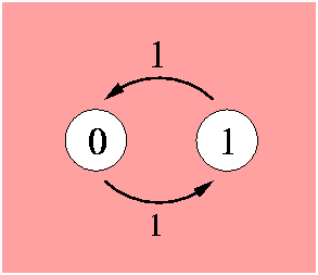
The position can be in its initial value (0) or in a different value (1). Both transitions are equally probable, this is indicated by the probability flow in each direction labeled as 1. The model is governed by the Markov property which states that the future behaviour of the process given its path only depends on its present state. Transitions from one state to the other can occur at any instant in time. A Markov process is determined by the transition rate matrix:
M := [ [-1,1], [1,-1] ]: print(M);
 -1  1
  1 -1
As the probability mass flowing from one state to the other is conserved, the columns sum to zero. The state probability vector P is a function of time t. The differential equation describing the change of state is the following:
P'(t) = alpha*M*P(t)
This is a system of coupled differential equations as P'(t) and P(t) are vectors and M is a matrix. The formal solution is given by:
        (alpha M t)
P(t) = e            P(0)
that describes the probability distribution of the states after time t given an initial probability distribution P(0). The factor alpha specifies the time unit, that is how fast or slow the transitions happen. The general solution to the differential equation can be expressed by
              (alpha l1 t)          (alpha l2 t)
P(t) = c1 V1 e             + c2 V2 e
where the li are the eigenvalues of M, Vi the corresponding eigenvectors and ci coefficients to be determined from the initial probabilities P(0). We compute now the eigenvalues and eigenvectors:
Eigenvalues(M,V); print(V);
[-2, 0]
  0.70710678 -0.70710678
 -0.70710678 -0.70710678
Note that the function Eigenvalues returns the eigenvalues and stores the the eigenvectors in the matrix V. Plugging the results into the general solution and using P(0)=[1,0] (i.e. no mutations have occurred at time zero) we can determine the coefficients ci leading to:
P(t) = [1/2 + 1/2 exp(-2 alpha t), 1/2 - 1/2 exp(-2 alpha t)]
To measure the amount of mutation in PAM units (Point Accepted Mutations, from Dayhoff et al.) alpha should be computed so that the expected number of mutations at time t=1 is 1/100:
1/2 - 1/2 exp(-2 alpha) = 1/100
alpha := -1/2*ln(49/50);
alpha := 0.01010135
and P(t) simplifies to
                     t               t
P(t) = [1/2 + 1/2 .98 , 1/2 - 1/2 .98 ]
The relation between t and real time is unknown and depends on the actual mutation rate (mutations per year). However, unless the mutation rate changes with time, t is strictly proportional to time.
When we have N positions with the same distribution, the distribution of the total number of mutations is a binomial distribution. The expected value of the total number of mutations is simply the product of N times the expected value of a single one. The variance of the distribution is also readily available. I.e.
                                  t
E[mutationsCount] = 1/2 N (1 - .98 )
                                    t          t
var[mutationsCount] = 1/4 N (1 - .98 ) (1 + .98 )
The following code computes the exact probability distribution at time t=20 (20 PAM). The binomial distribution has to be computed using logarithms to avoid overflows/underflows that will happen when very large factorials are computed.
N := 1000;
P := CreateArray(1..N+1):
pr := 1/2*(1-0.98^20);
for i from 0 to N do
    lnpr := LnGamma(N+1) - LnGamma(i+1) - LnGamma(N-i+1) +
        i*ln(pr) + (N-i)*ln(1-pr);
    P[i+1] := exp(lnpr)
od:
printf( 'expected: %.4f, variance: %.4f, std: %.4f\n',
    N*pr, N*pr*(1-pr), sqrt( N*pr*(1-pr) ) );
N := 1000
pr := 0.1662
expected: 166.1960, variance: 138.5749, std: 11.7718
check = sum(P)-1;
DrawPlot( P, axis );
check = -3.0842e-13
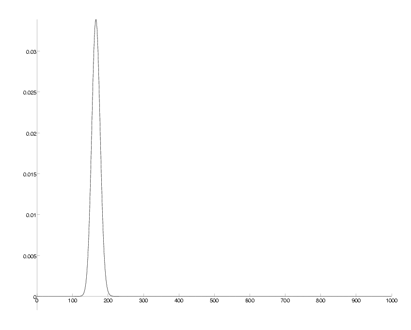
probability distribution for number of mutations at 20 PAM
Alternatively, we could solve the same problem with a completely coupled system where each state counts the number of mutations. In this case it makes little sense to use it, as its complexity is much higher. Still, there is the validation aspect and it is useful to have it in our toolbox for some variant where this technique will be needed. To describe the N positions we need N+1 states that will count how many positions have mutated. The diagram is:
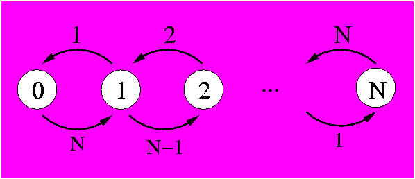
In the above figure it can be seen that each state (white circle) counts the number of mutations that have happened with its associated number. State 0 describes the system with no mutations. In state one, for example, one mutation has been observed. From this state, there are N-1 chances that in the next time step another mutation is observed, thus putting the system in state 2. There is also the possibility that in the next time step a mutation occurs on the same position as the 1 observed mutation. This would reverse the mutation back to its original state (as our system is binary) and thus we would be back at the state of 0 observable mutations.
The mathematics of a binary set of N positions is determined by the possible transitions. There are N+1 states, 0-mutations, 1-mutation, 2-mutations, ..., N-mutations. In an infinitesimal amount of time, transitions can only be made between states differing by 1 mutation so that the rate transition matrix is tridiagonal:
           / -N   1                      \
           |  N  -N   2                  |
           |     N-1 -N   3              |
       M = |            ...              |
           |                 -N  N-1     |
           |                  2  -N   N  |
           \                      1  -N  /
The differential equation describing the change of state with time is identical as the one for one position, but with dimension N+1 instead of 2.
P'(t) = alpha*M*P(t)
Analogue to the one-position-case, the solution is given by:
        (alpha M t)
P(t) = e            P(0)
that describes the probability distribution of the possible states after time t given an initial probability distribution P(0)=[1,0,0,0,...,0]. As an example and to check consistency, we will compute the values of the distribution for 20 PAM. This time we are not going to express P(t) in terms of the eigenvalues and eigenvectors of M. Instead use Darwin's facility to exponentiate matrices:
M := CreateArray(1..N+1,1..N+1):
for i to N do
    M[i,i+1] := i;
    M[i,i] := -N;
    M[i+1,i] := N-i+1
od:
M[N+1,N+1] := -N:
P20 := exp(M*alpha*20) * [1,seq(0,i=1..N)]:
We do not print the matrix M nor its exponential, as these matrices are very large. To compare the two probability vectors, we will compute the norm of the difference:
check := (P-P20)^2;
check := 3.7263e-27
To understand the relation between mutations and time we calculate the expected number of observable mutations (ev), as well as the 95% confidence intervals (plow and pup) for PAM distances up to 150 in increments of 1 PAM. We pre-compute the logarithms of the binomial coefficients to save repetitive computation.
MaxPam := 150;
upper := ev := lower := [[0,0]]:
lnBin := CreateArray(1..N+1):
for i from 0 to N do
    lnBin[i+1] := LnGamma(N+1) - LnGamma(i+1) - LnGamma(N-i+1)
od:
MaxPam := 150
Here we calculate the expected number of mutations at each PAM distance. The variable pam loops over each integer PAM distance. The expected value is accumulated in the list ev. The lower confidence level, plow is computed first by summing the bottom probabilities while they add 2.5% or less (half of 5%). Then the same is done for the upper probabilities, pup. These lines define the 95% confidence level swath.
for pam to MaxPam do
    pr := 1/2*(1-0.98^pam);
    for i from 0 to N do
        P[i+1] := exp( lnBin[i+1] + i*ln(pr) + (N-i)*ln(1-pr) )
    od:
    ev := append( ev, [pam,N*pr] );
    plow := pup := 0;
    for il to N+1 do
        if plow + P[il] >= 0.025 then break fi;
        plow := plow + P[il]
    od;
    lower := append( lower, [pam,il-1] );
    for iu from N+1 by -1 to 1 do
        if pup + P[iu] >= 0.025 then break fi;
        pup := pup + P[iu]
    od;
    upper := append( upper, [pam,iu-1] );
od:
bytes alloc=39600000, time=104.340
Once the expected value, and the upper and lower values of the 95% confidence level are found, they can be plotted for better visualization. Darwin's plotting function, DrawPlot accepts as input lists of x,y point and can also accept a list of objects to be plotted. A complete description can be obtained by typing ?DrawPlot in Darwin. We pick an arbitrary PAM value and print the expected count value, and the upper and lower 95% confidence levels.
lines := []:
PamLine := 20;
printf( 'at Pam %d, counts are between %d and %d 95%% of the time\n',
        PamLine, lower[PamLine+1,2], upper[PamLine+1,2] );
PamLine := 20
at Pam 20, counts are between 143 and 190 95% of the time
The first two lines below plot the vertical lines at 20 PAM, the expected, high and low values. Then we draw a horizontal line at 40% of the total counts (400 mutation), and the expected, high and low PAM values for this mutation count.
lines := append( lines,
    LTEXT(PamLine,lower[PamLine+1,2]-5,string(lower[PamLine+1,2]))):
lines := append( lines,
    RTEXT(PamLine-1,upper[PamLine+1,2],string(upper[PamLine+1,2]))):
CntLine := round(0.4*N);
for i1 to N-1 while
    not (upper[i1,2] <= CntLine and upper[i1+1,2] > CntLine) do od;
for i2 from 2 to N while
    not (lower[i2-1,2] < CntLine and lower[i2,2] >= CntLine) do od;
printf( 'at %d counts, Pam values are between %d and %d\n',
    CntLine, i1, i2 );
lines := append( lines, RTEXT(i1,CntLine+2,string(i1))):
lines := append( lines, LTEXT(i2,CntLine-10,string(i2))):
CntLine := 400
at 400 counts, Pam values are between 67 and 99
Finally we add some descriptive labels and plot the actual curves of the expected value and the upper/lower 95% confidence levels.
lines := append( lines,
    CTEXT(MaxPam/2,-20,'PAM distance'),
    CTEXT(-5,CntLine*0.6,'mutation count',angle=90),
    LINE(PamLine,0,PamLine,0.3*N),
    LINE(0,CntLine,MaxPam,CntLine) ):
DrawPlot( {lower,ev,upper,lines}, axis );
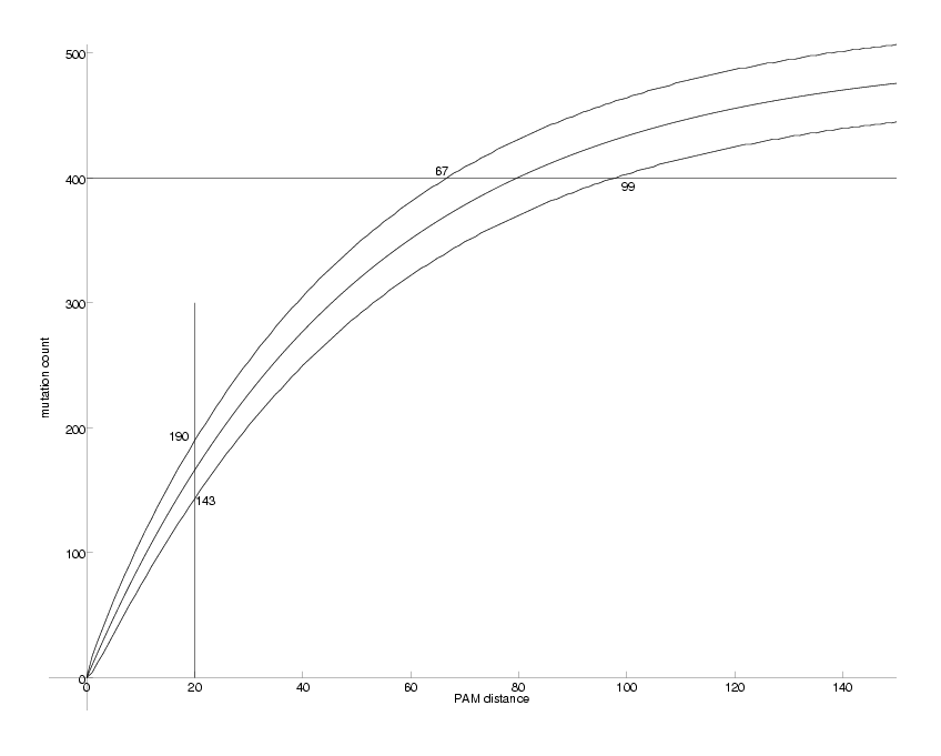
Observable Mutations as a Function of PAM distance
The middle curve shows the expected number of mutations resulting from a corresponding PAM distance. The two curves above and below mark the 95% confidence interval for the mutation count. e.g. for PAM = 20, we expect between 143 and 190 out of 1000 mutations 95% of the time. The problem we want to solve is the inverse: we observe the mutation count and want to estimate the PAM distance. This is equivalent to inverting the middle curve. e.g. if we observe 400 mutations (out of 1000) these could have been produced by PAM distances between 67 and 99. In this case the middle curve can be easily inverted:
      ln(1 - 2 i/N)
pam = -------------
            49
         ln(--)
            50
pam := ln( 1 - 2*CntLine/N ) / ln(0.98);
pam := 79.6645
Instead of a mathematical or numerical inversion of the function (which may not be possible for more complicated cases), we can use maximum likelihood estimation of the PAM distance. The maximum likelihood estimate must coincide with the inversion of the middle curve. If p(t) is the probability of a simple mutation the likelihood of observing i out of N is:
                   i           (N - i)
binomial(N, i) p(t)  (1 - p(t))
The logarithm of the likelihood differentiated with respect to t is:
  /d      \           /d      \   /d      \
i |-- p(t)|   (N - i) |-- p(t)|   |-- p(t)| (i - N p(t))
  \dt     /           \dt     /   \dt     /
----------- - ----------------- = ----------------------
   p(t)           1 - p(t)           p(t) (1 - p(t))
The solution of the above coincides with our previous formula for the pam distance, as expected. The second derivative of the log likelihood is the negative inverse of the variance. Doing a bit of algebra we find that:
                  i (N - i)
Var(pam) = 4 --------------------
                49 2          2
             ln(--)  (N - 2 i)  N
                50
i := CntLine;
PamVar := 4*i*(N-i) / (ln(49/50)^2*(N-2*i)^2*N);
i := 400
PamVar := 58.8020
and if express the variance in terms of the distance:
           /50\(2 pam)
           |--|        - 1
           \49/
Var(pam) = ---------------
                   49 2
              N ln(--)
                   50
PamVar := ((50/49)^(2*pam)-1)/N/ln(49/50)^2;
PamVar := 58.8020
We are now ready to show the main features/problems of molecular clocks based on mutations. Although this analysis was done for a very simple model, the conclusions extend to most other cases.
| I | It is clear that the results are only approximate. Even from a set of 1000 positions we have very large uncertainties, even for lower PAM distances. However, if we had infinitely many positions, the results would be exact. |
| II | While the uncertainty decreases with more positions, it does so with an inverse square root law. i.e. we need 4 times more points to decrease the uncertainty intervals by 2. |
| III | Saturation is the term used to describe the situation that happens when the count of mutations is high enough to make the PAM range predictions infinite. Again, this happens only because we have a finite number of positions. |
| IV | The computation of the expected number of mutations is based on time. As an abstract unit of time we use PAM units. So the x-axis is a time-axis. |
| V | A binary case, as shown here, carries less information than a quaternary case (DNA). So working with more possible states will improve the estimates (shown next). |
| VI | For small distances, say up to 20 PAM, the curve is almost a straight line. If the curve were always a straight line, estimating PAM could be done directly from the counts. But it is not a straight line, even for infinitely many positions. So inverting the curve is always needed to get proper time estimates. |
| VII | The error in estimating PAM distances from counts increases by two factors. First, the variance of the actual counts increases with PAM distances (the swath gets wider to the right). Secondly, as the curve has a lower slope, the horizontal cut covers a large uncertainty region. These two effects add together to make higher PAM estimates less accurate. |
| VIII | Finally, it should be noticed that in this example the confidence interval (upper/lower curves) is only 95%. Safer intervals, e.g. 99.9%, would roughly increase the swath by about 50%. |
We will now extend the idealized model from binary to quaternary. That is, every position has four possible states. This will allow us to model DNA under the simplified assumption that all mutations are equally likely. In the current literature, this is called the Jukes-Cantor model. Here we solve it exactly and study is behaviour in detail.
The analysis is still simple enough that we can generalize it to a k-ary system without much more complication. The previous case falls under k=2, and the DNA model under k=4. To model this k-ary system, given that all states behave identically, we will consider again two states, the original position and any of the k-1 possible mutations. For a position which has not mutated, as in the binary case, it will mutate to a different state. The difference with the binary case is for a mutated position, it can mutate to another different position (k-2 out of k-1) or to the original state (1 out of k-1). The transition diagram for k=4 is as follows:
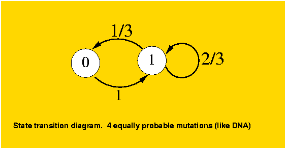
The mutation matrix is:
             / -1   1/(k-1)  \
         M = |               |
             \  1  -1/(k-1)  /
Using similar arguments as for the binary case we can produce from M and P(0) the solution vector:
                       t                   t
              (k - 1) r   k - 1   (k - 1) r
P(t) = [1/k + ----------, ----- - ----------]
                  k         k         k
If time is in PAM units, then
                k
r = 1 - 1/100 -----
              k - 1
the pam estimation based on i mutation counts is:
                i k
      ln(1 - ---------)
             N (k - 1)
pam = -----------------
            ln(r)
and the variance of the estimate is:
                   2
                  k  i (N - i)
Var(pam) = ---------------------------
                2                  2
           ln(r)  (N (k - 1) - i k)  N
and if express the variance in terms of the distance:
             (-pam)        (-pam)
           (r       - 1) (r       + k - 1)
Var(pam) = -------------------------------
                                 2
                  N (k - 1) ln(r)
We can now compute the graphs again, with almost the same code, the only change is the general formula for pr:
k := 4;
r := 1 - k/100/(k-1);
upper := ev := lower := [[0,0]]:
for pam to MaxPam do
    pr := (k-1)/k*(1-r^pam);
    for i from 0 to N do
        P[i+1] := exp( lnBin[i+1] + i*ln(pr) + (N-i)*ln(1-pr) )
    od:
    ev := append( ev, [pam,N*pr] );
    plow := pup := 0;
    for il to N+1 do
        if plow + P[il] >= 0.025 then break fi;
        plow := plow + P[il]
    od;
    lower := append( lower, [pam,il-1] );
    for iu from N+1 by -1 to 1 do
        if pup + P[iu] >= 0.025 then break fi;
        pup := pup + P[iu]
    od;
    upper := append( upper, [pam,iu-1] );
od:
k := 4
r := 0.9867
lines := []:
PamLine := 40;
printf( 'at Pam %d, counts are between %d and %d 95%% of the time\n',
        PamLine, lower[PamLine+1,2], upper[PamLine+1,2] );
PamLine := 40
at Pam 40, counts are between 283 and 340 95% of the time
The first two lines below plot the vertical lines at 40 PAM, the expected, high and low values. Then we draw a horizontal line at 60% of the total counts (600 mutation), and the expected, high and low PAM values for this mutation count.
lines := append( lines,
    LTEXT(PamLine,lower[PamLine+1,2]-5,string(lower[PamLine+1,2]))):
lines := append( lines,
    RTEXT(PamLine-1,upper[PamLine+1,2],string(upper[PamLine+1,2]))):
CntLine := round(0.6*N);
for i1 to N-1 while
    not (upper[i1,2] <= CntLine and upper[i1+1,2] > CntLine) do od;
for i2 from 2 to N while
    not (lower[i2-1,2] < CntLine and lower[i2,2] >= CntLine) do od;
printf( 'at %d counts, Pam values are between %d and %d\n',
    CntLine, i1, i2 );
lines := append( lines, RTEXT(i1,CntLine+2,string(i1))):
lines := append( lines, LTEXT(i2,CntLine-10,string(i2))):
lines := append( lines,
    CTEXT(MaxPam/2,-25,'PAM distance'),
    CTEXT(-5,CntLine*0.6,'mutation count',angle=90),
    LINE(PamLine,0,PamLine,0.4*N),
    LINE(0,CntLine,MaxPam,CntLine) ):
CntLine := 600
at 600 counts, Pam values are between 107 and 138
This code plots the actual curves of the expected value, upper and lower curves.
DrawPlot( {lower,ev,upper,lines}, axis );
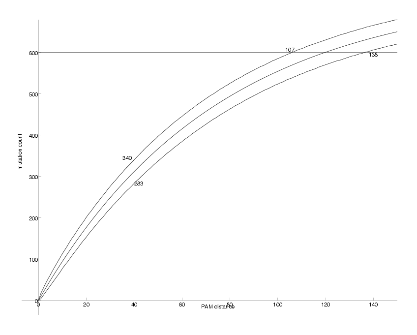
Observable DNA Mutations as a Function of PAM distance
We can now compare the figure above with the one we produced for k=2. There are two main differences. First, while for k=2 the counts saturate at about 440, they do so at about 620 for k=4. Second, the uncertainties for k=4 are smaller, i.e. the upper and lower curves run closer to the middle one. The explanation for this observations is that the quaternary case carries more information than the binary one.
Please cite as:
@techreport{ Gonnet-orthologues,
        author = {Gina M. Cannarozzi and Gaston H. Gonnet},
        title = {Idealized Mutational Clocks},
        month = { November },
        year = {2005},
        number = { xxxxx },
        howpublished = { Electronic publication },
        copyright = {code under the GNU General Public License},
        institution = {Informatik, ETH, Zurich},
        URL = { http://cbrg.inf.ethz.ch/bio-recipes/IdealMut/code.html }
        }
© 2006 by Gina Cannarozzi and Gaston Gonnet, Informatik, ETH Zurich
Last updated on Sat Apr 1 21:04:45 2006 by GNA