A big field of research in Computational Biology concentrates on constructing phylogenetic trees. Often we have the difficult situation where a long time ago two speciation events have occurred in a very small period of time. This bio-recipe describes how we can compute a confidence level for such a problematic case in a parsimony framework.
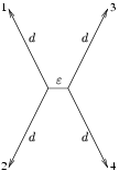
The situation just described can be simplified in a quartet which has a short middle branch and four similarly long branches to the leafs, as indicated in the figure below.
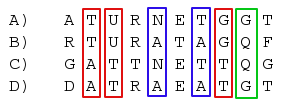
There are three different possible unrooted trees with four leafs. In a parsimony framework, we can count from the four aligned sequences the number of sites, that give support for each of them. By looking at the alignment example below, we can immediately say that the 3 red sites give support for a tree where A and B are on one side of the tree and C and D on the other. The blue sites support a tree where A, C and B, D are neighbors where as the green site indicates, that A, D and B, C would be the right tree. All the other sites do not favor any tree and thus can be ignored.
We want to conclude which tree is actually the right one, even though it is clear, that we will always find sites that give support for any of the three trees. One would expect, that the longer the middle branch is, the more sites will indicate the right tree.
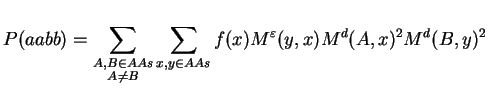
To study this problem, we assume a case with 4 species all having the same PAM distance d from the middle branch and a middle branch having a PAM distance epsilon. We assume a Markovian model of evolution and we will compute the probabilities of all the configurations. First, we need to know, how often we expect to see a site supporting one of the three trees. We assume that all sites in the multiple sequence alignment are independent and mutate at the same rate. Thus, we can compute the support probability for the figure above:
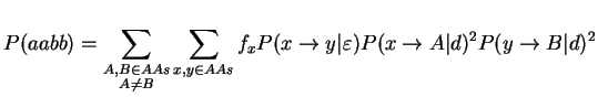
where fi is the natural frequency of the ith amino acid and P(x --> A|d) stands for the probability that the amino acid x mutates to A given a PAM-distance of d. The probability of getting support for one of the false trees can be computed in an analogous manner. The following function will compute the probabilities that a site supports each of the three possible trees.
CreateDayMatrices():
# the logPAM1 matrix and AF (AA-frequencies) are now defined

SupportProb := proc( eps:positive, d:positive )
    M_d   := exp( d*logPAM1 ):
    M_eps := exp( eps*logPAM1 ):

    supProb := CreateArray(1..3):
    for x to 20 do
        for y to 20 do
            t := AF[x]*M_eps[y,x];
            for A to 20 do
                for B to 20 do
                    if A=B then next fi;
                    supProb[1] := supProb[1] + t * M_d[B,y]^2 * M_d[A,x]^2;
                    supProb[2] := supProb[2] + t * M_d[A,y]*M_d[B,y]*M_d[A,x]*M_d[B,x];
                od:
            od:
        od:
    od:
    supProb[3] := supProb[2];
    return(supProb);
end:
Because the probability of getting the 3th tree is equal to the 2nd, we just have to compute it once. To get a feeling of these probabilities, we try eps=1 and d=20:
supProb := SupportProb(1,20);
supProb := [0.01012627, 0.00577918, 0.00577918]
As we can see, the support sites occur rarely. The correct support occurs in 1% of the sites and the incorrect support roughly 0.58% each. Next, we try to compute the probability of finding the right tree. We assume that the sites are all independent, hence we could model each site as the outcome of a quadrinomial distributed random variable. Since the probability of getting support for at least one of the trees is small, we will approximate the three interesting outcomes as independently distributed Poisson variables. Thus, the probability of identifying the right tree is equal to the cumulative distribution of finding more support sites for the correct tree than for the other two. Mathematically this can be expressed as
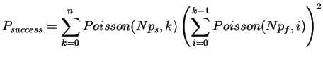
Due to this simplification we are now able to compute the success probability very efficiently (in linear time), since we can reuse the calculation of the inner sum for each k. To avoid over- and underflows when evaluating the exponentials and factorials, we use the logarithms:
SuccessProb := proc(N, supProb:list(positive) )
    pSuc := cum := 0:
    lmda := N*supProb;
    for k to N do
        cum := cum + exp( -lmda[2] + (k-1)*ln(lmda[2]) - LnGamma(k) );
        pSuc_k := exp(-lmda[1] + k*ln(lmda[1]) - LnGamma(k+1));
        s := pSuc_k * cum^2;
        if k>lmda[1] and s < DBL_EPSILON*pSuc then
            # if we are beyond the peak and the value for k is
            # smaller than the machine precision we can stop.
            break;
        fi;
        pSuc := pSuc + s;
    od:
    return(pSuc);
end:
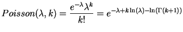
To see the influence of the middle branch on the success probability we can evaluate this function for different PAM distances. The plot below shows the success and the failure probability at a fix distance d=20 PAM and variable epsilon for N=10000 observed sites.
sucPts := []:
for eps from 0.000001 to 1.3 by 0.1 do
    freqs := SupportProb(eps,20);
    sucPts := append( sucPts, [eps, SuccessProb(10000, freqs)] );
od:

failPts := [ seq([z[1], 1-z[2]], z=sucPts) ]:
DrawPlot( {sucPts,failPts}, axis );
Success probability versus PAM-distance of the middle branch.
As expected, we observe that the success probability gets higher the longer the middle branch is. On the other hand, the success probability approaches 1/3 for very small epsilon, which matches the case where the tree degenerates into a star and hence all three trees are equally likely.
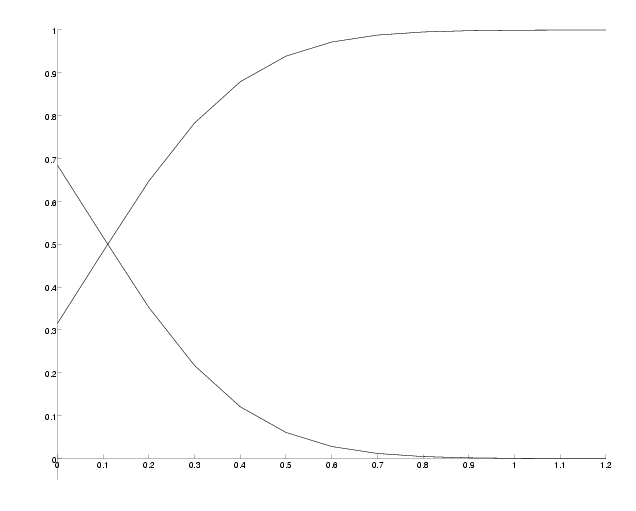
N, the number of observed sites has also an influence on the success probability. Since the support probabilities are so small, we have to choose N sufficiently big to observe enough sites giving any support information. To demonstrate this, we will compute the success probability for different N at epsilon=0.2, where the success probability was around 0.6 in the previous example.
supProb := SupportProb(0.2,20):
sucPts := [seq([i/4,SuccessProb(10^(i/4),supProb)], i=8..24)]:
xlabel := [CTEXT( 4, -0.05, 'log10( number of sites )' )]:
DrawPlot( {sucPts,xlabel}, axis );
Success probability versus number of sites.
In this section we will study the effect of an outgroup species on the success probability. An outgroup is a species that is farther related to all the other species than the others are among themselves. We are interested to determine the influence on the ability to decide for the correct tree depending on the distance of the outgroup. The scenario is exactly the same except that this time, we will vary the distance d of one species and keep epsilon constant. For that, we change our previous defined function "SupportProb" as follows:
SupportProb := proc( eps:positive, d:positive, d_out:positive )
    CreateDayMatrices():

    M_d   := exp( d*logPAM1 ):
    M_out := exp( d_out*logPAM1 ):
    M_eps := exp( eps*logPAM1 ):

    supProb := CreateArray(1..3):
    for x to 20 do
        for y to 20 do
            t := AF[x]*M_eps[y,x];
            for A to 20 do
                for B to 20 do
                    if A = B then next fi:
                    supProb[1] := supProb[1] + t * M_d[A,x]^2 * M_d[B,y]*M_out[B,y];
                    supProb[2] := supProb[2] + t * M_d[A,x]*M_d[B,x]*M_d[A,y]*M_out[B,y];
                od:
            od:
        od:
    od:
    supProb[3] := supProb[2];
    return(supProb);
end:
Warning: procedure SupportProb reassigned
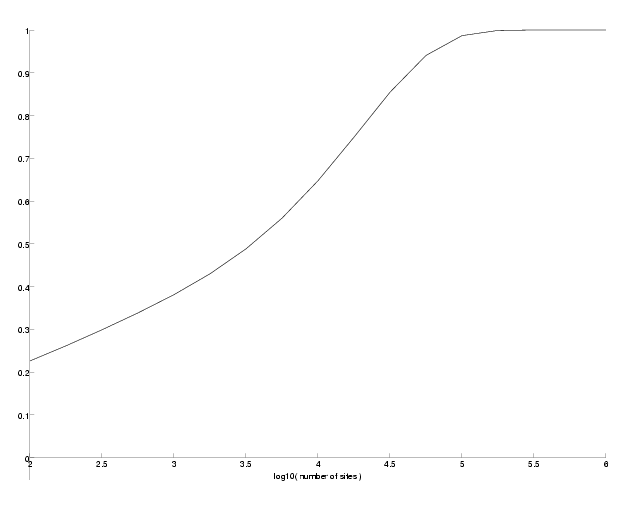
The only difference in the function is in the computation of the support probability where we use the mutation matrix at a PAM distance of the outgroup for one of the leafs. Note that it actually makes a small difference in the support probabilities on which side of the tree the outgroup lies. Since theses differences are really small, we just randomly choose one side. The following program computes the success probabilities for an outgroup at a PAM-distance between 20 and 60 for three different epsilon.
curves := labels := []:
for eps in [0.1,0.5,1.0] do
    pts := []:
    for d_out from 20 to 60 by 5 do
        freqs := SupportProb(eps, 20, d_out);
        pts := append( pts, [d_out, SuccessProb(10000, freqs)] );
    od:
    curves := append( curves, pts);
    labels := append( labels, LTEXT(pts[2,1],pts[2,2]+0.01,sprintf('eps=%.1f',eps)) );
od:
DrawPlot( {op(curves),labels}, axis );
Success probability versus PAM-distance of the outgroup.
As we can see, the success probabilities decrease the farther the outgroup is located for all epsilon. However, the decrease is not very large.
A very expensive part in terms of computational time in the previous programs is the computation of the support probabilities. It is of order O(n4). In this section, we describe how one can compute the support probability faster by applying linear algebra. Our main goal is to get rid of the summations over x and y. (A and B would in principle also be possible, but since A and B are related (have to be different), this would be much more complicated.)
The support probability can be written using mutation matrices:
By defining U(i,j) := Md(i,j)2 and rearranging of terms we obtain
By doing a matrix multiplication of U and Meps, we avoid the summation over y. The next step follows the same concept: we try to replace the summation over x by a matrix multiplication. For that, we need to define F as a diagonal matrix holding the natural amino acid frequencies f:
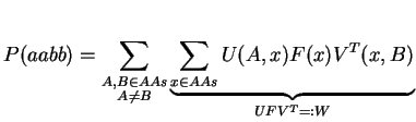
Note, that we have to transpose V for the multiplication. Finally, it just remains the summation over A and B:
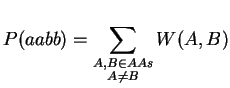
The complexity of this improved algorithm is of order O(n3) as the matrix-matrix multiplication is the most expensive operation. Since the matrix-matrix multiplication is done in the kernel, we can expect the computation to be a lot faster. The following code shows the difference:
SupportProbSlow := proc( eps:positive, d:positive )
    M_d   := exp( d*logPAM1 ):
    M_eps := exp( eps*logPAM1 ):

    supProb := 0;
    for x to 20 do
        for y to 20 do
            t := AF[x]*M_eps[y,x];
            for A to 20 do
                for B to 20 do
                    if A=B then next fi;
                    supProb := supProb + t * M_d[B,y]^2 * M_d[A,x]^2;
                od:
            od:
        od:
    od:
    return(supProb);
end:

SupportProbFast := proc( eps:positive, d:positive )
    M_d   := exp( d*logPAM1 ):
    M_eps := exp( eps*logPAM1 ):

    U := [seq( [seq( M_d[i,j]^2, j=1..20)], i=1..20)];
    Vt := transpose(U*M_eps);

    # multiplication of F with Vt
    Vt := [seq( AF[i]*Vt[i], i=1..20)];
    W := U*Vt;

    supProb := sum(sum(W)) - sum(W[i,i],i=1..20);
    return(supProb);
end:

Set(gc=1e7): gc():
tSlow := time():
supProbSlow := SupportProbSlow(1,20):
tSlow := time() - tSlow;

gc():
tFast := time():
supProbFast := SupportProbFast(1,20):
tFast := time() - tFast;
tSlow := 0.2100
tFast := 0
checkDiff := supProbFast - supProbSlow;
checkDiff := 1.5092e-16
As we can see, both procedures compute the same result (except for roundoff errors), but the improved one computes the result a lot faster. Unfortunately, there does not exist such a simple rearrangement for the support probabilities of getting the wrong trees.
© 2006 by CBRG Group, Informatik, ETH Zurich
Please cite as:
@techreport{ Gonnet-quartetconfidence,
        author = {Adrian M. Altenhoff and Gaston H. Gonnet},
        title = {Computing Confidence Levels for Quartets},
        month = { October },
        year = {2006},
        number = { 537 },
        howpublished = { Electronic publication },
        copyright = {code under the GNU General Public License},
        institution = {Informatik, ETH, Zurich},
        URL = { http://www.biorecipes.com/QuartetConfidence/code.html }
        }
Last updated on Wed Nov 8 11:04:46 2006 by AA