This bio-recipe shows how to classify viruses using their k-nucleotide (di-, tri- and tetra-nucleotide) frequencies. It also shows how we can build a phylogenetic tree of the viruses. The content is based on the research by Kurt Tobler & Mathias Ackermann, Institute of Virology, University of Zurich.
We have put together a virus genome database. Our goal is to build a phylogenetic tree of these viruses. First, let us load the database.
ReadDb('/home/darwin/v2/source/bio-recipes/VirusClassification/viruses.db');
DNA file(/home/darwin/v2/source/bio-recipes/VirusClassification/viruses.db(
702100), 49 entries, 695010 bases)
We want to classify the viruses based on their k-nucleotide frequencies. Research has shown that dinucleotide frequencies are similar for related organisms and different for unrelated organisms. Furthermore, the frequencies are relatively constant over the whole genome, in both coding and non-coding regions of DNA. Hence, the vector of k-nucleotide frequencies is a signature of the genome.
The standard method of phylogenetic analysis is to construct trees from multiple sequence alignments (MSA). However, that approach suffers from the disadvantage that we have to limit the analysis to parts of the DNA which can be reliably aligned, for example coding regions. Naturally, we have to know the coding regions of the DNA, and we have to make an arbitrary choice of which regions to compare. Different regions can lead to different trees. Furthermore, finding a multiple sequence alignment for long regions of many organisms is computationally very intensive. However, the main problem by this method is the quality of the MSA. In the case of dinucleotide analysis, these problems do not exist.
To show the method, we start by looking at the nucleotide and dinucleotide frequencies of one single virus, namely SARS. First, we create a function that calculates the k-nucleotide frequencies of a DNA sequence s.
CalcFreq := proc(s: string, k: posint);
    freq := CreateArray(1..4^k);
    n := length(s)-k+1;
    for i to n do
We encode a k-nucleotide as a number base 4. For example, AAA -> 0 and TTTT -> 256.
        knuc := 0;
        for j to k do
            knuc := 4*knuc + NToInt(s[i+j-1]) - 1; od;
        knuc := knuc + 1;
        freq[knuc] := freq[knuc] + 1;
    od;
    freq / n;
end:
Next, we locate the SARS genome in the database.
s := Sequence(SearchID('SARS'));
s := ATATTAGGTTTTTACCTACCCAGGAAAAGCCAACCAACCTCGATCTCTTG ..(29751).. AAAAAAAAAAA
We calculate the nucleotide frequencies and print them.
NF := CalcFreq(s, 1):
print('Nucleotide frequencies:');
for i to 4 do
    printf('%s    %f\n', IntToN(i), NF[i]); od;
printf('The nucleotide frequencies add to %f\n', sum(NF));
Nucleotide frequencies:
A    0.285066
C    0.199657
G    0.207959
T    0.307317
The nucleotide frequencies add to 1.000000
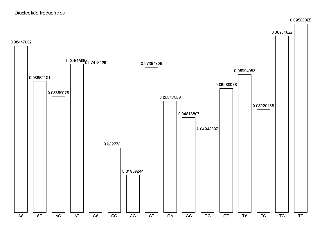
Finally, we calculate the dinucleotide frequencies and show them in a histogram.
diNF := CalcFreq(s, 2):
labels := CreateArray(1..16):
for i to 4 do
    for j to 4 do
        a := 4*(i-1) + j;
        labels[a] := IntToN(i) . IntToN(j); od; od;
DrawHistogram(diNF, labels, Title='Diucleotide frequencies');
#ViewPlot();

The observed frequency of a dinucleotide XY is not the same as the expected frequency of XY, which we can express as fXfY. As an example, we compare the observed and expected frequency of the dinucleotide AA.
diNF[1];
NF[1] * NF[1];
0.08447059
0.08126265
We will use the bias between observed and expected frequencies to classify the viruses. This bias can be calculated in various ways: as an odds ratio, as the logarithm of the odds ratio, as the deviation from a normalized Poisson distribution etc. Here we choose odds ratio, since it has been experimentally shown to be a good measure for phylogeny. The bias is calculated as b = fobs/fexp, where fobs=fXY and fexp=fXfY.
OddsRatio := proc(Fobs: list, Fexp: list);
    n := length(Fobs);
    bias := CreateArray(1..n);
    for i to n do
        bias[i] := Fobs[i] / Fexp[i]; od;
    bias;
end:

CalcBias := proc(Fobs: list, NF: list, method: string);
    n := length(Fobs);
    k := ln(n) / ln(4);
    Fexp := CreateArray(1..4^k, 1);
    for i to n do
        j := i-1;
        to k do
            Fexp[i] := Fexp[i] * NF[mod(j,4)+1];  j := floor(j/4) od; od;
    BiasFunction := symbol(method);
    if nargs >= 4 then
        BiasFunction(Fobs, Fexp, args[4..nargs]);
    else
        BiasFunction(Fobs, Fexp);
    fi;
end:
As an example, let us calculate this bias for the dinucleotides of SARS.
diNucBias := CalcBias(diNF, NF, 'OddsRatio'):
print('Dinucleotide bias:');
for i to 4 do
    for j to 4 do
        a := 4*(i-1) + j;
        printf('%s%s    %f\n', IntToN(i), IntToN(j), diNucBias[a]): od; od;
Dinucleotide bias:
AA    1.039476
AC    1.168768
AG    0.993398
AT    0.857931
CA    1.302831
CC    0.822144
CG    0.459831
CT    1.200282
GA    0.952573
GC    1.160101
GG    0.935021
GT    0.984059
TA    0.798459
TC    0.850771
TG    1.401140
TT    1.012561
We need to calculate this bias for all the viruses in the database. The result will be stored in the matrix diNucBias, which will be used soon.
n := DB['TotEntries']:
diNucBias := CreateArray(1..n, 1..4^2):
for i to n do
    s := Sequence(Entry(i)):
    NF := CalcFreq(s, 1):
    diNF := CalcFreq(s, 2):
    diNucBias[i] := CalcBias(diNF, NF, 'OddsRatio'):
od:
In order to create a phylogenetic tree, we need to know the evolutionary distance between the organisms in our population. This distance is defined as the euclidean distance of the k-nucleotide bias of two organisms a and b. For example, the dinucleotide distance between the first and the second organism in our database is:
sqrt((diNucBias[1]-diNucBias[2])^2);
0.7145
For the phylogenetic tree, we need the distances and variances of all pairs of organisms.
CalcDistances := proc(v: list)
    n := length(v);
    dist := CreateArray(1..n, 1..n);
    for i to n-1 do
        for j from i+1 to n do
            dist[i, j] := dist[j, i] := sqrt((v[i]-v[j])^2); od; od;
    dist;
end:

CalcVariances := proc(v: list(list));
    n := length(v);
    vmean := sum(Flatten(v)) / (n*(n-1));
    v*vmean;
end:

dist := CalcDistances(diNucBias):
We also need labels for the tree nodes.
GetLabels := proc(ID: string);
    n := DB['TotEntries'];
    labels := CreateArray(1..n);
    for i to n do
        labels[i] := SearchTag(ID, Entry(i)); od;
    labels;
end:

labels := GetLabels('ID'):
When generating the phylogenetic tree, we will use the built-in function MinSquareTree. It will start with a random tree and adapt it to our data. In order to improve the result, we run MinSquareTree several times, each one with a new random tree, and finally choose the best tree generated.
CreateTree := proc(dist, labels)
    global MinLen, MST_Qual;
    bestq := DBL_MAX;
    oldpr := printlevel;    printlevel := 0;
    MinLen := 0;
    vari := CalcVariances(dist);
    to 10 do
        t := MinSquareTree(dist, vari, labels, Random):
        if MST_Qual < bestq then
            bestq := MST_Qual;
            bestt := t;
        fi;
    od;
    printlevel := oldpr;
    MST_Qual := bestq;
    bestt;
end:

t := CreateTree(dist, labels):
#DrawUnrootedTree(t, 'Phylogenetic tree of viruses. Built from dinucleotide data. ' . sprintf('    MST_Qual=%f', MST_Qual));
cls := []:
for i to DB[TotEntries] do cls := append(cls, SearchTag(LA,Entry(i))[1] ) od:
DrawTree( t, Unrooted, OrderLeaves=cls, Clusters=cls, LengthFormat='' );
ViewPlot();
DrawColorShape expects a 1st argument, t:Leaf, found: [Leaf(IBV,-0.3887,22),
85.5405, 64.8237, 72.3895, 72.0127]
Error, (in LeafLab) invalid arguments
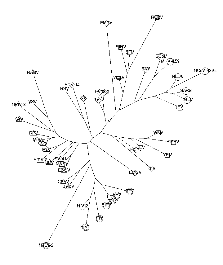
As we can see from the picture, the classification works quite well. The Corona, Flavi, Retro, Toga and Falvi viruses are all clustered together in the tree. All except one of the Mononega viruses are also together. The Picorna viruses are quite spread out, possibly because they have relatively inhomogeneous genomes. Here is the list of the viruses and their descriptions:
print('Label  Short     Description');
for e in Entries() do
    desc := SearchTag('DE', e):
    desc := If(length(desc)<=60, desc, desc[1..60]):
    printf(' %-4s  %-9s %s\n', SearchTag('LA', e), SearchTag('ID', e), desc);
od;
Label  Short     Description
 c4    BCoV      Bovine coronavirus isolate BCoV-ENT, complete genome
 m9    BDV       BDU04608 Borna disease virus V, complete genome
 x1    BVDV      BVDCG Bovine viral diarrhea virus complete genome
 m1    CDV       AF164967 Canine distemper virus strain A75/17, complete geno
 x2    CSFV      HCU45477 Hog cholera virus strain Riems, complete genome
 n1    EAV       TOEAV Equine arteritis virus (EAV) RNA genome
 m5    EBOV      Zaire Ebola virus, complete genome
 p8    EMCV      EVCGAA Encephalomyocarditis virus complete RNA genome
 r2    FFV       FFVAJ3851 feline foamy virus RNA genome
 r4    FIV       FIVCG Feline immunodeficiency virus complete genome
 p6    FMDV      PIFMDV2 Foot and mouth disease virus (FMDV-O1K) RNA for poly
 . . . . (26 output lines skipped) . . . .
 m7    SeV       SNDT5RCG Sendai virus strain mutant T-5 revertant, complete
 t4    SFV       ALSFV42S Semliki forest virus 42S RNA genome
 r6    SiFV      SFU04327 Simian foamy virus SFVcpz, complete genome
 t2    SINV      SINCG Sindbis virus (hrsp and wild-type strains) complete ge
 m11   SV-41     SV41RNA Simian virus 41 genes NP, P, M, F, HN and L
 f4    TBEV      Tick-borne encephalitis virus, complete genome
 c5    TGEV      TGA271965 Transmissible gastroenteritis virus complete genom
 p2    ThV       TMEGDVCG Theiler murine encephalomyelitis, complete genome
 t3    VEEV      EEVCOMGEN Venezuelan equine encephalitis virus, complete gen
 m3    VSV       VSVCG Vesicular stomatitis Indiana virus, complete genome
 f3    WNV       WNFCG West Nile virus RNA, complete genome
 f2    YEV       Yellow fever virus, complete genome
We will try to improve the tree by studying trinucleotides and tetranucleotides. They are calculated in the same way as dinucleotides.
triNucBias := CreateArray(1..n, 1..4^3):
tetraNucBias := CreateArray(1..n, 1..4^4):
for i to n do
    s := Sequence(Entry(i)):
    NF := CalcFreq(s, 1):
    triNF := CalcFreq(s, 3):
    tetraNF := CalcFreq(s, 4):
    triNucBias[i] := CalcBias(triNF, NF, 'OddsRatio'):
    tetraNucBias[i] := CalcBias(tetraNF, NF, 'OddsRatio'):
od:
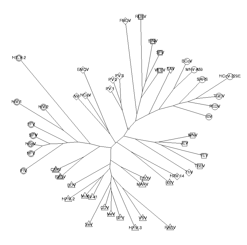
We build a tree from the trinucleotide data.
t := CreateTree(CalcDistances(triNucBias), labels):
#DrawUnrootedTree(t, 'Phylogenetic tree of viruses. Built from trinucleotide data' . sprintf('    MST_Qual=%f', MST_Qual));
DrawTree( t, Unrooted, OrderLeaves=cls, Clusters=cls, LengthFormat='' );
ViewPlot();
DrawColorShape expects a 1st argument, t:Leaf, found: [Leaf(IBV,-1.2247,22),
88.7950, 73.0908, 70.9763, 79.7575]
Error, (in LeafLab) invalid arguments
The tree from the tetranucleotide data looks like this.
t := CreateTree(CalcDistances(tetraNucBias), labels):
#DrawUnrootedTree(t, 'Phylogenetic tree of viruses. Built from tetranucleotide data' . sprintf('    MST_Qual=%f', MST_Qual));
DrawTree( t, Unrooted, OrderLeaves=cls, Clusters=cls, LengthFormat='' );
ViewPlot();
DrawColorShape expects a 1st argument, t:Leaf, found: [Leaf(MHV-A59,-3.3318,26),
95.2419, 44.7201, 80.4434, 48.2343]
Error, (in LeafLab) invalid arguments
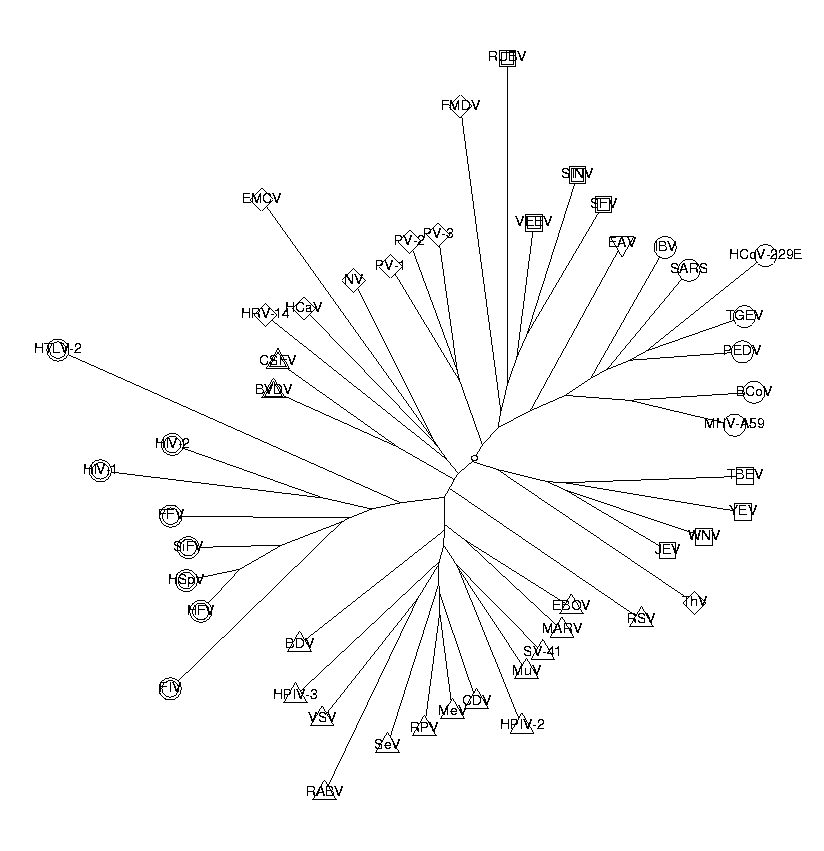
It is clear that increasing the dimension k of the k-nucleotides increases the selectivity of the pattern, and hence the distances should be more accurate. So in principle, the higher the k value, the more information we capture and the more reliable the results should be. However, this is counterbalanced by the background noise of the distances, which is proportional to O(4^k). I.e. in every component of the vector there is some expected error. In the case of the Poisson model, this error has variance 1. As we compute the distance between two vectors, these errors add together, and because of the exponential size of the vectors, the error becomes very significant for k>3. The additional noise, which acts as an added value to each distance, is reflected in the trees themselves which become more corona-shaped (which can be seen in the images above). Furthermore, the additional noise, which makes all the distances larger by an additive constant, makes the tree fitting by least squares numerically better. This is quite disconcerting, as a better fit means worse trees. We choose the trinucleotide results as the best compromise between information and noise.
In the trees that we have produced so far, the coronaviruses are clearly clustered together on their own branch. SARS is among the coronaviruses in each tree, so we draw the conclusion that SARS is a corona virus. However, the internal topology of the coronaviruses differs from tree to tree. A possible reason for this is that the minimum square tree is calculated based on the all-against-all distances, and a global optimum is searched, even if this is not optimal for the local virus groups. As a result, the relative positions of the coronaviruses may be affected by the distances of the other virus groups. By studying the coronaviruses alone, this problem is avoided.
We will do the same analysis as above for the coronaviruses only. This is easy now that we already have the functions.
ReadDb('/home/darwin/v2/source/bio-recipes/VirusClassification/coronaviruses.db');
n := DB['TotEntries']:
diNucBias := CreateArray(1..n, 1..4^2):
triNucBias := CreateArray(1..n, 1..4^3):
tetraNucBias := CreateArray(1..n, 1..4^4):
for i to n do
    s := Sequence(Entry(i)):
    NF := CalcFreq(s, 1):
    diNF := CalcFreq(s, 2):
    triNF := CalcFreq(s, 3):
    tetraNF := CalcFreq(s, 4):
    diNucBias[i] := CalcBias(diNF, NF, 'OddsRatio'):
    triNucBias[i] := CalcBias(triNF, NF, 'OddsRatio'):
    tetraNucBias[i] := CalcBias(tetraNF, NF, 'OddsRatio'):
od:

labels := GetLabels('ID'):

diNucDist := CalcDistances(diNucBias):
t := CreateTree(diNucDist, labels):
#DrawUnrootedTree(t, 'Coronaviruses. Built from dinucleotide data' . sprintf('   MST_Qual=%f', MST_Qual));
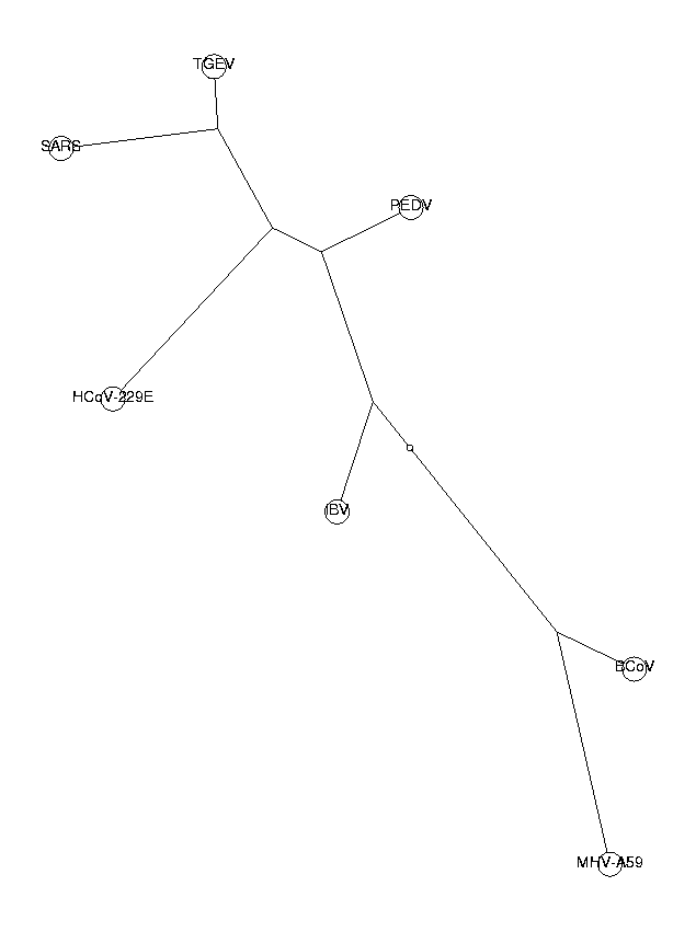
DrawTree( t, Unrooted, LengthFormat='' );
ViewPlot();
DNA file(/home/darwin/v2/source/bio-recipes/VirusClassification/coronaviruses.db
(204872), 7 entries, 203680 bases)
triNucDist := CalcDistances(triNucBias):
t := CreateTree(triNucDist, labels):
#DrawUnrootedTree(t, 'Built from trinucleotide data' . sprintf('   MST_Qual=%f', MST_Qual));
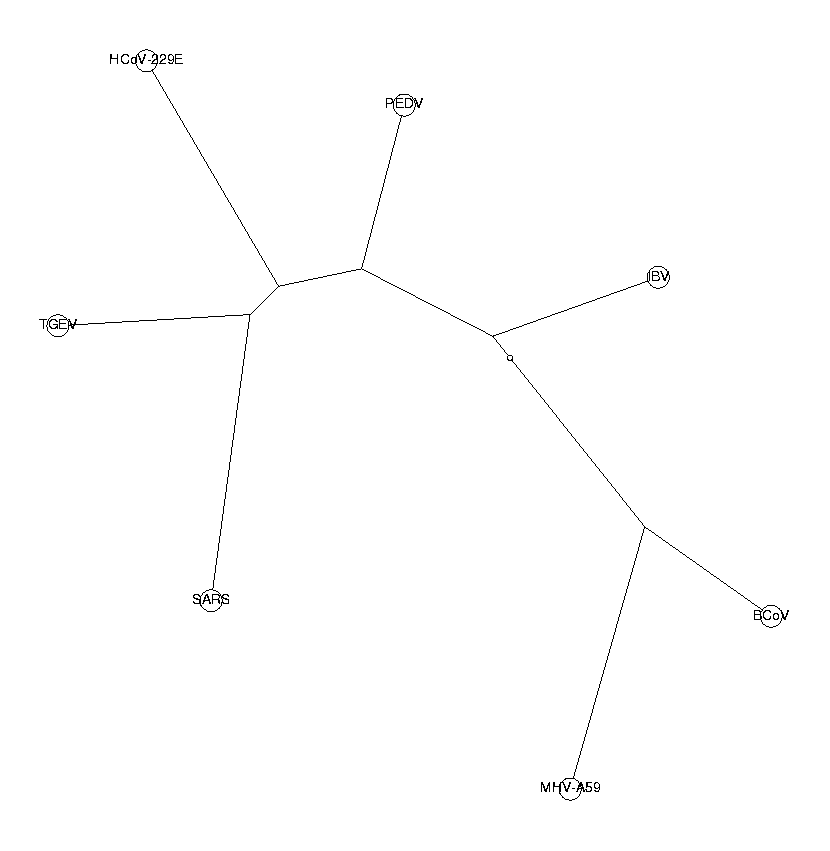
DrawTree( t, Unrooted, LengthFormat='' );
ViewPlot();
tetraNucDist := CalcDistances(tetraNucBias):
t := CreateTree(tetraNucDist, labels):
#DrawUnrootedTree(t, 'Coronaviruses. Built from tetranucleotide data' . sprintf('   MST_Qual=%f', MST_Qual));
DrawTree( t, Unrooted, LengthFormat='' );
ViewPlot();
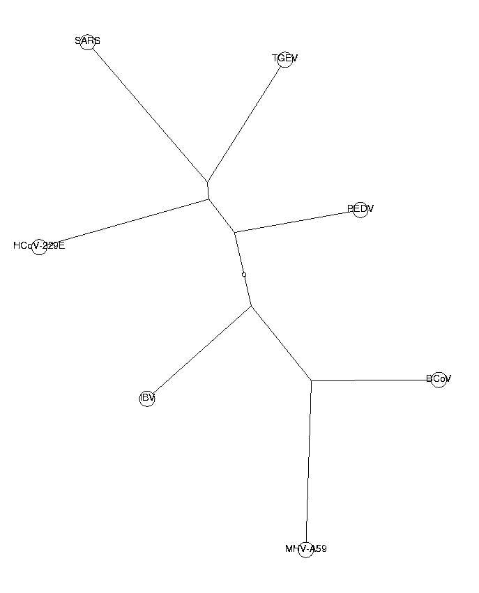
The trees from di-, tri- and tetranucleotides all have the same topology. This is a good indication that our phylogenetic trees are reliable. The three neighboring coronaviruses of SARS (HCoV-229E, PEDV and TGEV) are known to belong to group I of coronaviruses. From these trees, we draw the conclusion that SARS also belongs to this group. SARS is in our tree closest to TGEV, so we hypothesize a close relationship to the TGEV virus.
Instead of odds ratios, we can use the Poisson distribution as a bias measure.
PoissonDistr := proc(Fobs: list, Fexp: list, N: posint);
    n := length(Fobs);
    bias := CreateArray(1..n);
    for i to n do
        bias[i] := (Fobs[i] - Fexp[i]) / (N * Fexp[i] * (1-Fexp[i])); od;
    bias;
end:

triNucBias := CreateArray(1..n, 1..4^3):
for i to n do
    s := Sequence(Entry(i)):
    NF := CalcFreq(s, 1):
    triNF := CalcFreq(s, 3):
    triNucBias[i] := CalcBias(triNF, NF, 'PoissonDistr', length(s)):
od:
t := CreateTree(CalcDistances(triNucBias), labels):
#DrawUnrootedTree(t, 'Tree from trinucleotide data using Poisson distr.' . sprintf('    MST_Qual=%f', MST_Qual));
DrawTree( t, Unrooted, LengthFormat='' );
ViewPlot();
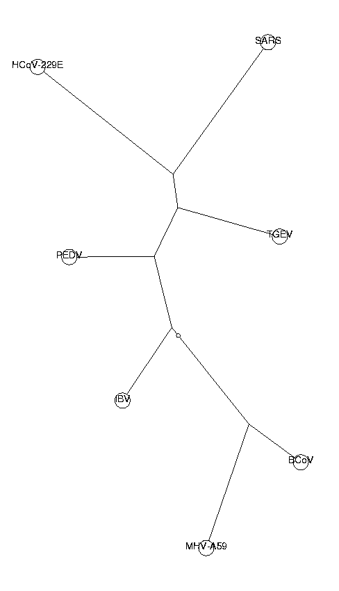
The topology of this tree is identical to the ones produced by the odds ratio method. SARS is placed among group I of coronaviruses. The fact that two different methods generate the same topology makes our results more reliable.
To further test our conclusion, we create a phylogenetic tree using optimal pairwise alignments. The pairwise alignments are based on an RNA mutation matrix derived from the 50 viruses.
CreateDayMatrices(ViralRNA):
Since these alignments take a long time to compute, we will try to load them from a file. If the file is not found, the alignments will be computed and saved.
OpenReading('/home/darwin/v2/source/bio-recipes/VirusClassification/AllAllCorona.res');
if not type(AllAll,matrix({0,Alignment})) then
    AllAll := CreateArray(1..n, 1..n):
    for i to n do
        for j from i+1 to n do
            AllAll[i,j] := AllAll[j,i] := Align(Entry(i),Entry(j), DMS);    lprint(i,j); od od;
    OpenWriting('AllAllCorona.res');
    printf('AllAll := %A:\n', AllAll);
    OpenWriting(previous);
fi;
Now we are ready to create the tree based on the pairwise alignments.
t := PhylogeneticTree( [ seq(Sequence(Entry(i)), i=1..n)],
    [ seq(SearchTag(ID,Entry(i)), i=1..n ) ],
    Distance, AllAll):

DrawUnrootedTree(t, 'Corona viruses, distance tree');
#ViewPlot();
DrawUnrootedTree(Tree(Leaf(IBV,-36.1492,3),0,Tree(Tree(Tree(Leaf(BCoV,-36.0179,1
),-19.2553,Leaf(MHV-A59,-36.3088,4),1),-3.1255,Leaf(SARS,-36.6293,6),0.9999),
-0.4116,Tree(Tree(Leaf(HCoV-229E,-37.1136,2),-8.4540,Leaf(PEDV,-34.7944,5),
0.9904),-6.7172,Leaf(TGEV,-36.0311,7),1),1)),Corona viruses, distance tree)
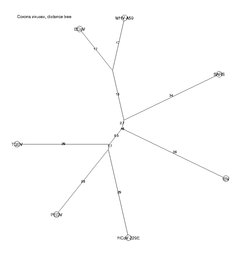
This method does not confirm our results, since SARS is here placed on a branch of its own, not among the group I of coronaviruses. Hence we have two methods (k-nucleotides and pairwise alignments) which give different results. We will investigate this in more detail.
It is interesting to see which virus is most related to SARS. We compare the distances from the pairwise alignments to the distances from the k-nucleotides. For the PAM distances we can compute their variances, so we have an estimate of the confidence. We show 95% confidence intervals. For the euclidean distances of the k-nucleotideswe do not have an estimate of the variance. The distances have been scaled so that the minimum distances coincide.
First, we prepare a list of PAM distances and variances between SARS and each of the other coronaviruses. We are not interested in the distance between SARS and itself, so we treat that case specially.
PAMdist := CreateArray(1..n-1):
PAMvari := CreateArray(1..n-1):
i := 0:
for z in AllAll[6] do
    if z = 0 then next fi:
    i := i+1:
    PAMdist[i] := z[PamDistance]:
    PAMvari[i] := z[PamVariance]:
od;
The k-nucleotide distances are normalized. Also here we need to exclude the distance between SARS and itself.
NormalizeDistances := proc(dist, m);
    d := dist[6];
    d := [op(d[1..5]), d[7]];
    k := m / min(d);
    d*k;
end:

m := min(PAMdist):
diNucDist := NormalizeDistances(diNucDist, m):
triNucDist := NormalizeDistances(triNucDist, m):
tetraNucDist := NormalizeDistances(tetraNucDist, m):
Finally, we print the results.
printf('             PAM distance     dinucl. dist.    trinucl. dist.   tetranucl. dist\n');
j := 0:
for i to 7 do
    if i = 6 then next fi;
    j := j + 1:
    printf('%9s    %.1f +- %.2f  %12.1f  %15.1f  %15.1f\n', SearchTag('ID', Entry(i)), PAMdist[j], 1.96*sqrt(PAMvari[j]), diNucDist[j], triNucDist[j], tetraNucDist[j]); od;
             PAM distance     dinucl. dist.    trinucl. dist.   tetranucl. dist
     BCoV    68.0 +- 1.93         249.9            125.5            104.7
HCoV-229E    70.0 +- 2.16         161.0             86.0             77.3
      IBV    77.0 +- 2.12         169.7             97.1             88.9
  MHV-A59    65.0 +- 1.98         294.9            138.8            110.4
     PEDV    71.0 +- 2.17         126.6             81.6             77.1
     TGEV    70.0 +- 2.15          65.0             65.0             65.0
According to the pairwise alignments method, SARS is closest to MHV. However, note that the difference in distance between SARS and the other viruses is quite small, especially when considering the confidence interval. In the case of k-nucleotides, the differences are much clearer, which could indicate that the clustering is more reliable. Furthermore, the distances coincide for di-, tri- and tetranucleotides.
In order to check the reliability of the pairwise alignment method, we print the alignment between SARS and the closest neighbor: MHV.
print(AllAll[6][4]);
SARSlength := length(Sequence(Entry(6))):
SARSaligned := AllAll[6][4][Length2]:
printf('\n%d nucleotides out of %d (%.1f%%) in the SARS genome were used in the local pairwise alignment.\n', SARSaligned, SARSlength, 100*SARSaligned/SARSlength);
lengths=14199,14181 simil=13023.9, PAM_dist=65, identity=56.4%
ID=MHV-A59   DE=Mouse hepatitis virus strain MHV-A59 C12 mutant, complete genome

ID=SARS   DE=SARS coronavirus TOR2, complete genome
TGTTGCCAATATGCTTCCAGCTTTTACGTTACTGCGATTTTACATCGTGGTGACAGCTATGTATAAGGTCTATTGTCTTT
|.|||...|.|||...||.|.||.|.|..|..|..|..|.||||||.|..|..|..||.|.||..|..|.|........|
TATTGTACAAATGGCACCCGTTTCTGCAATGGTTAGGATGTACATCTTCTTTGCTTCTTTCTACTACATATGGAAGAGCT

GTAGACATGTTATGTATGGATGTAGTAAGCCTGGTTGCTTGTTTTGTTATAAGAGAAACCGTAGTGTCCGTGTTAAGTGT
.|...|||.|.|||.||||.||.|......|...||||.||.|.||.||||||.|.||.|||......||.|||.|||||
ATGTTCATATCATGGATGGTTGCACCTCTTCGACTTGCATGATGTGCTATAAGCGCAATCGTGCCACACGCGTTGAGTGT

 . . . . (701 output lines skipped) . . . .
.|.||.|||||.||.|..|.........|........|.||....||||||||||||||.||.||.|||.|.|||.....
ATTTTCTGGAGGAACACAAATCCTATCCAGTTGTCTTCCTATTCACTCTTTGACATGAGCAAATTTCCTCTTAAATTAAG

TGGTACGGCTGTTGTTAGCCTTAAACCAGACCAAATAAATGACTTAGTCCTCTCCTTGATTGAGAAGGGCAAGTTATTAG
.||.||.|||||..|....|||||.....|.|||||.|||||..|..|....||..|..|.||.||.||.|.|.|..|..
AGGAACTGCTGTAATGTCTCTTAAGGAGAATCAAATCAATGATATGATTTATTCTCTTCTGGAAAAAGGTAGGCTTATCA

TGCGTGATACACGCAAAGAAGTTTTTGTTGGCGATAGCCTAGTAAATGTCAAA
|..|.||.|....||.||..||..||....|.||||..||.||.||...|.||
TTAGAGAAAACAACAGAGTTGTGGTTTCAAGTGATATTCTTGTTAACAACTAA

14181 nucleotides out of 29751 (47.7%) in the SARS genome were used in the local pairwise alignment.
The number of identical nucleotides is quite low, and less than half of the nucleotides were used in the alignment.
Our result that SARS belongs to group I of coronaviruses contradicts the result presented in (Rota, 2003 and Merra, 2003), where it is concluded that SARS does not belong to any of the three known coronavirus groups, but instead forms a new group. Their analysis was based on MSAs of 4-5 proteins that are common for the coronaviruses. There is strong evidence for both methods, and we do not claim that ours has to be the correct one. The purpose of this bio-recipe is rather to show that there are two scientifically sound methods that give different results.
© 2009 by Markus Friberg, Informatik, ETH Zurich
Please cite as:
@techreport{ Friberg-virusclassif
        author = {Markus Friberg},
        title = {Virus Classification using <i>k</i>-nucleotide Frequencies},
        month = { May },
        year = {2003},
        number = { 401 },
        howpublished = { Electronic publication },
        copyright = {code under the GNU General Public License},
        institution = {Informatik, ETH, Zurich},
        URL = { http://www.biorecipes.com/VirusClassification/code.html }
        }
Last updated on Thu Mar 12 12:20:47 2009 by MF